
Network measurement techniques have been mostly developed independently from protocols and, therefore, typically build upon externally visible semantics. One example of this is TCP sequence numbers and acknowledgements, which can be used to derive a flow’s round-trip time (RTT).
Unfortunately, fully encrypted transport protocols, such as QUIC, make these techniques impossible as the protocol semantics are no longer visible to on-path observers.
For this purpose, QUIC introduces a dedicated special-purpose bit, the spin bit, which can be used to derive a flow’s RTT and whose effectiveness has already been shown.
Read: Explicit passive measurability and the QUIC Spin Bit
Technical details, as well as ethical considerations surrounding the spin bit have already been addressed on the APNIC Blog. In this post, I want to highlight work my colleagues and I at RWTH Aachen University recently presented in our ANRW paper, which sought to evaluate the performance of four spin bit cousins L, Q, R, and T. I’ll touch on how these different techniques allow network operators to observe packet loss on different parts of their network and discuss their accuracy.
Spin bit cousins
This work stems from an ongoing discussion in the IETF IPPM working group regarding additional measurement bits to enable packet loss measurements. The four proposals — L, Q, R, and T — provide different possibilities to grasp packet loss.
The L-Bit uses end-host loss detection and for each packet deemed lost in the network, it simply sets the L-Bit on one outgoing packet. Thus, any on-path observer can simply count the number of L-marked packets to determine the number of lost packets.
In contrast, the other three variants require an observer to first count marked packets and then compare them to expected values.
The Q-Bit, for example, encodes a square wave signal and an observer can measure the number of packets having a Q-marking received in each interval. Packet loss can then be derived by comparing this number to the original length of the square wave.
The R-Bit uses the same technique but instead uses the received Q wavelength as its own outgoing wavelength, thus reporting back the number of incoming Q-markings.
The T-Bit reflects a train of packet-markings with a dynamic size several times between the server and the client, and an observer can then compare the number of observed packet-markings each time the packet train passes through.
Please refer to our paper or the IPPM draft for a more detailed explanation of the spin bit cousins.
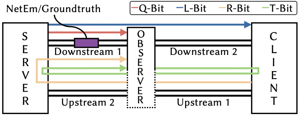
Due to their design, the different techniques observe packet loss on different parts of the network as shown in Figure 1. This, additionally, allows observers to segment the network in different ways and locate the cause of the error. While this is also of interest for network operators, this post focuses on the measurement accuracy of the different approaches.
How accurate are they?
We studied the packet loss measurement accuracy in a Mininet-based testbed and use an extended version of the aioquic QUIC implementation that features implementations for the four proposed mechanisms and modifies QUIC’s short header so that we can capture all mechanisms at the same time.
Random Loss
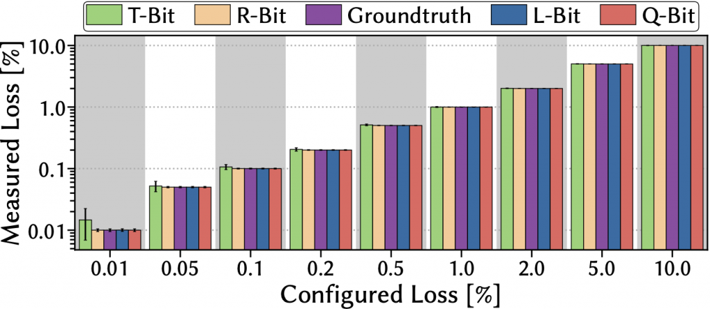
Figure 2 shows the average loss rate that the four techniques measure when facing increasing random loss rates that we configured using Linux’s traffic control netem. As can be seen, all approaches can accurately track the loss although the T-Bit struggles slightly for lower loss percentages.
Taking a closer look (Figure 3) at the temporal behaviour of one example measurement run with a configured loss rate of 1 %, we can quickly identify the reasons why this is the case.
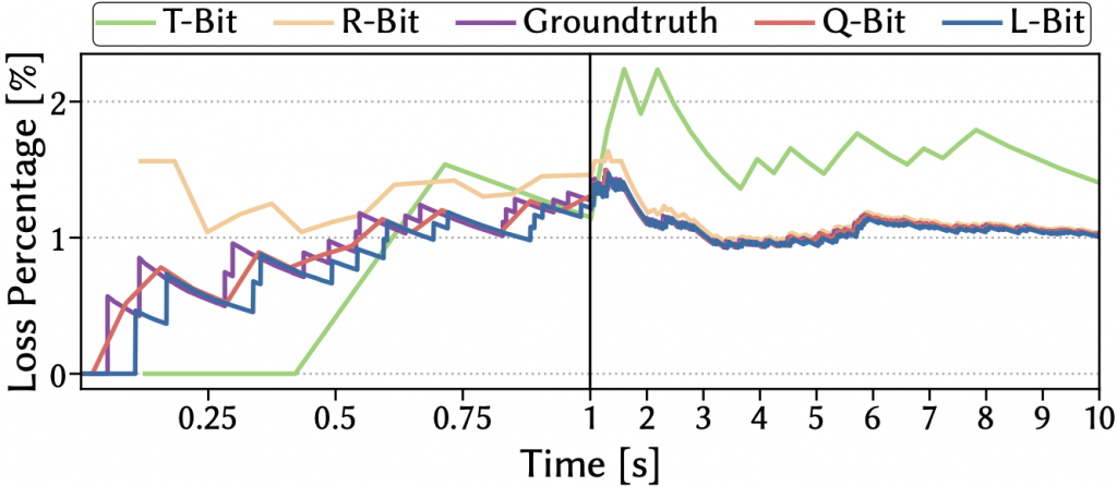
The Q-Bit and L-Bit closely follow the groundtruth as their design allows for immediate measurements.
The R-Bit, on the other hand, first has to wait until the first iteration of Q-markings has been completed before it can start its own measurements, meaning that it misses the start of a connection.
Finally, the phase-based approach of the T-Bit makes it regularly miss parts as it includes pause phases and can only measure loss occurring at certain times. Consequently, it produces fewer readings and additionally also fluctuates significantly around the groundtruth.
Burst packet loss
All approaches are also robust to small average burst packet loss (Figure 4), which we configured using the simple Gilbert model.
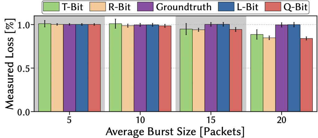
However, performance for most starts deteriorating quickly for increasing burst sizes and only the L-bit remains close to the groundtruth as it is the only approach without algorithmic phases that directly leverages the end-hosts’ loss detection. For all the others, too large burst losses that cancel out entire algorithmic periods will ultimately cause them to miss the real loss.
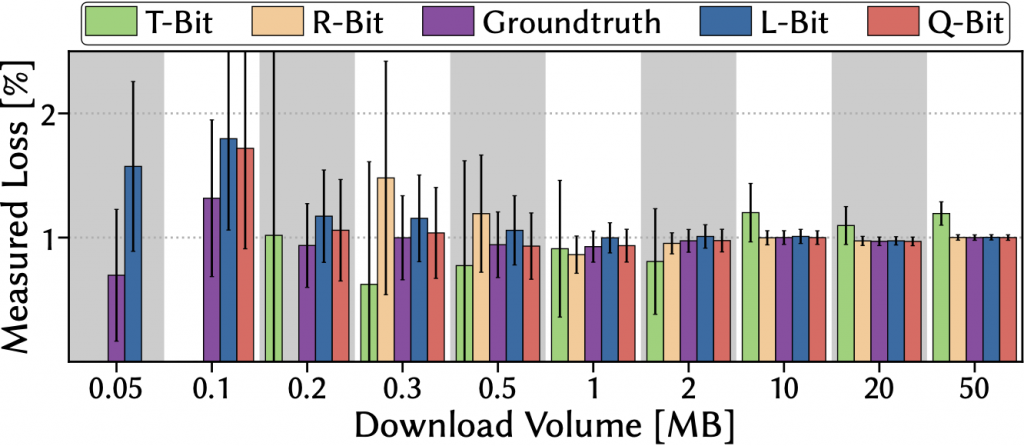
Flow length
Studying the usefulness of the approaches for real traffic, we have found that connections need to have certain minimum durations to enable sensible measurements. When configuring a constant random loss rate of 1% and then performing downloads of different volumes, the earlier finding of different starting points for the measurements again materializes as the L-Bit is the first to produce measurements with the Q-Bit following closely behind. In our setting (Figure 5), a download volume of about 1 to 2MB already allowed for quite stable measurements, indicating the general practicality of these approaches to real Internet traffic.
The path to real deployment
The prospect of enabled network measurements is promising for network operators as they rely on accurate information on the status for the operation and management of their networks.
Unfortunately, the recently standardized spin bit can only rarely be seen spinning in today’s production traffic — Google and Facebook, two of the largest shareholders in QUIC traffic, do not use the feature. Consequently, it is dubious whether additional bits might see adoption in reality.
What is needed are clear incentives for big players such as CDN providers to deploy these new techniques. Unfortunately, these benefits are currently only seen on the network operators’ side.
Are you a network operator yourself and thinking about leveraging the spin bit? Or are you using QUIC traffic and have on purpose decided against using the spin bit? We are interested in your opinion on this topic. Please leave us a comment or drop us an email!
Contributor: Jan Rüth
Ike Kunze is a PhD student at the Chair of Communication and Distributed Systems at RWTH Aachen University in Germany.
The views expressed by the authors of this blog are their own and do not necessarily reflect the views of APNIC. Please note a Code of Conduct applies to this blog.