

The North American Network Operators Group (NANOG) can trace its beginnings to the group of so-called ‘Mid Level’ networks that acted as feeder networks for the NSFNET, the backbone of the North American Internet in the first part of the 1990s. NANOG’s first meeting was held in June 1994, and NANOG held its 95th meeting 30 years later, in Arlington, Texas in October of this year.
Here’s my take on a few presentations that caught my attention during this three-day meeting.
5G, fibre and Wi-Fi
The last 45 years have been a wild ride in the communications industry, and Len Bozack’s presentation at NANOG 95 illustrated some highlights in both cellular radio and Ethernet over this period (Figure 1). Ethernet has lifted in capacity from 10Mbps common bus to 800Gbs. The cellular systems have progressed through kilobits per second analogue systems, to today’s 5G systems that have 2.3 billion subscriptions worldwide. The mobile service market sees USD 244 billion in annual spend, out of a total of some USD 462 billion per year in network infrastructure and devices. The balance, about USD 212 billion per year is largely due to investments in core and access services in the fixed line networks. This is clearly big business!
In the mobile world, 5G is gaining the dominant position in most regional markets, but interestingly, the annual growth in data volumes has been slowing down since its peak in 2019. By 2025, the annual growth rate in 5G network data volumes is down to 19% from a high of over 90% in mid-2018. This could be a sign of market saturation in many markets for mobile services, as well as some stability in service usage patterns in recent years.
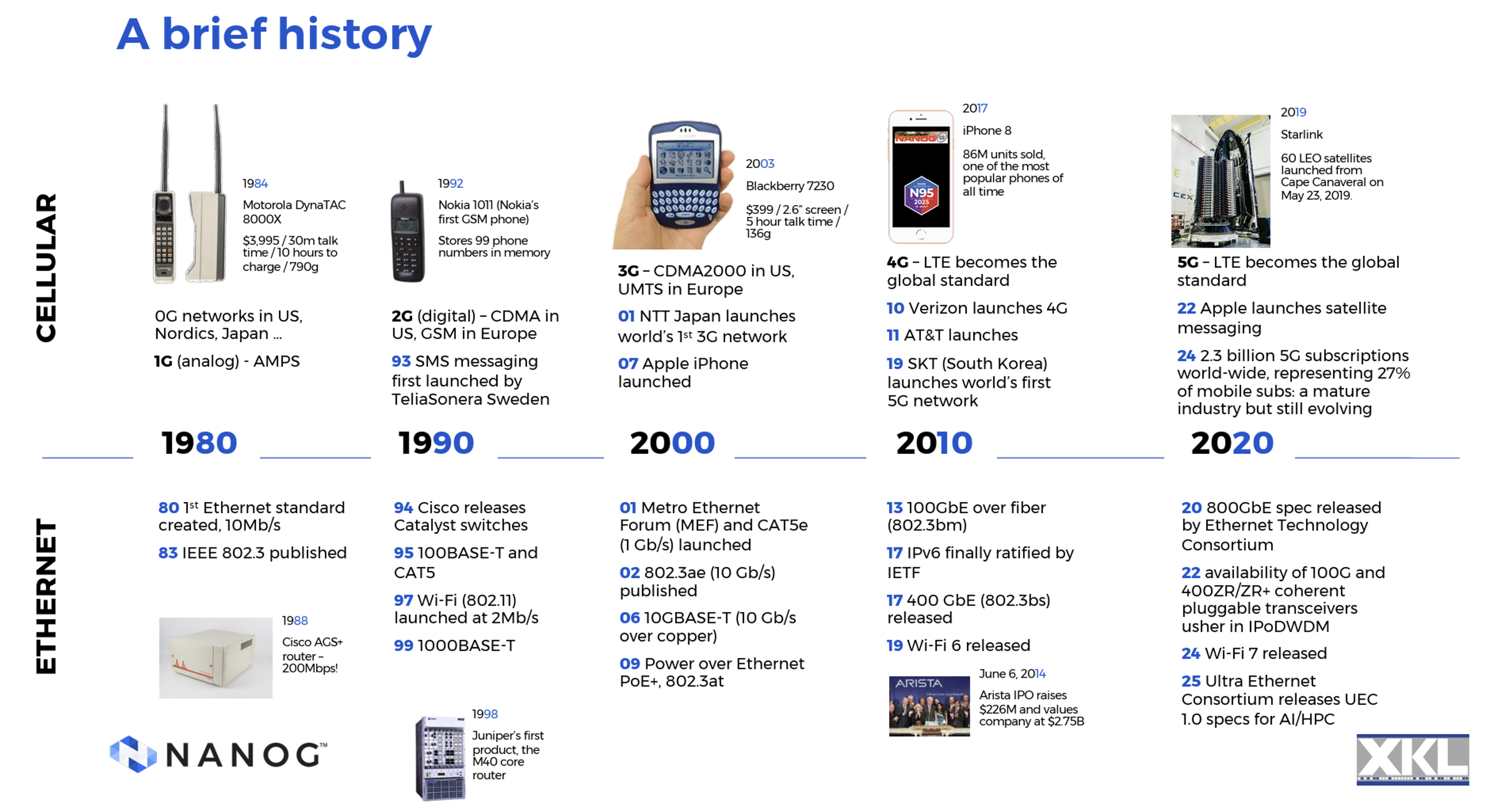
There has been a similar evolution in Wi-Fi technology, despite the lack of commercial service operators, something that has been a feature of the evolution of the mobile cellular service. The initial Wi-Fi technology was a 11Mbps service using Quaternary Phase Shift Keying (QPSK) encoding within the 2.4GHz band. Successive evolution of Wi-Fi has increased the signal density, increased the number of channels and opened up new radio bands.
| Year | Gen | Speed | Technology |
| 1999 | 1 | 11Mbps | 20Mhz QPSK 2.4GHz |
| 2003 | 2 | 54Mbps | 20MHz multi-channel 64QAM 5GHz |
| 2004 | 3 | 54Mbps | 20MHz multi-channel 64QAM 2.4/5GHz |
| 2009 | 4 | 600Mhz | 40MHz channel bonding, 4×4 MIMO, 64QAM, 2.4/5GHz |
| 2013 | 5 | 78Ghz | 80/160Mhz channel bonding, 4DL MU-MIMO, 256 QAM |
| 2019 | 6 | 9.6GHz | 80/160Mhz channel bonding, OFDMA, UL, 4DL MU-MIMO, 1024 QAM |
| 2024 | 7 | 23GHz | 320MHz Channel Bonding, MLO, MRU, R-TWT, 4096 QAM |
Wi-Fi is now a USD 35.6B market, showing an 11% annual growth rate. Seamless Roaming (single mobility domains), Multi Access Point (AP) coordination, and Enhanced Edge Reliability make Wi-Fi 8 a whole lot closer to Mobile 5.5/6G, albeit in a very limited domain.
The same advances in digital signal processing that have been fundamental to the performance improvements in 5G and Wi-Fi have also been applied in Hybrid Fibre Coax (HFC) deployments. Data Over Cable Service Interface Specification (DOCSIS) 4.0 using 2GHz of bandwidth and 4096 quadrature amplitude modulation (QAM) allows for a capacity of 10Gbps downstream and 6Gbps upstream.
HFC networks are very power intensive due to the amount of equipment in the outside network, including amplifiers and nodes. While the power efficiency of HFC systems has doubled in the past five years, fibre deployments consume less than half the power for comparable capacity. Fibre networks have a construction cost of USD 59 per km using underground conduits, and one-third of that cost using aerial fibre. XGS-PON splitters can deliver 10Gps per port.
I found Figure 2 from this presentation particularly interesting.
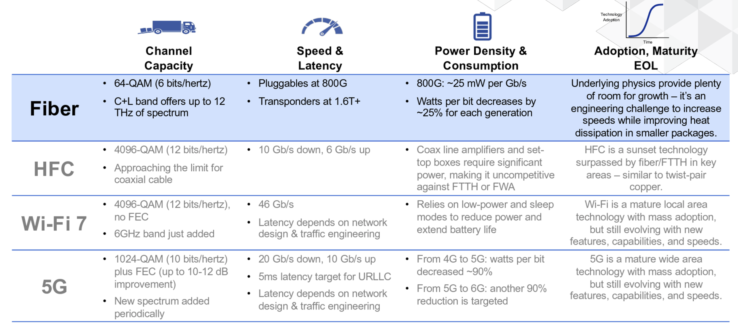
The future is, as usual, somewhat unclear. The mobile cellular markets are looking to open up the millimetre wavelength spectrum (92 to 300Ghz), labelled as part of 6G. However, these elevated frequency radio signals have almost no penetrative ability, so such a service would be a constrained short-range line-of-sight scenario. The economic model that can sustain the higher network costs with the higher base station density is very unclear.
Wi-Fi 8 does not represent any fundamental increases in speed, but improvements in power management may extend battery life in low-power devices. HFC is at its technology end-of-life in most markets, with little in the way of further enhancements anticipated. Current fibre systems can support 800G with a power budget of 25mW per Gbps. Smaller electronics need to be balanced again heat dissipation in the transponders.
Radio is a shared space, and the available spectrum is limited. As we shift into higher frequencies, we gain in available capacity, but lose out in terms of penetration, and therefore impaired utility. Cable-guided signals are not so limited, but this greater capability comes at a higher capital cost of installation and limited flexibility once it’s installed.
Presentation: 5G, Fiber, and Wi-Fi. The IP Takeover is (Almost) Complete – Len Bosack, XKL
BGP route leaks
Route leaks are challenging to detect. A ‘leak’ is a violation of routing policy where routes are propagated beyond their intended scope. It’s not Border Gateway Protocol (BGP) acting incorrectly. BGP itself is not the problem. The issue is normally a configuration mishap where the operator-determined controls that are normally placed on BGP route propagation fail to act as intended (see RFC 7908 for an extended exposition on Route Leaks).
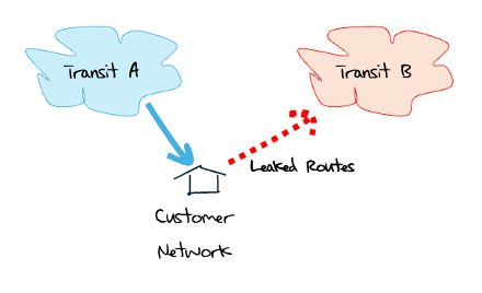
A common leak is a multi-homed stub network advertising one provider’s routes to the other (Figure 3). Not only is this cross traffic essentially unfunded, the traffic is rerouted along paths that are inadequately dimensioned for the volume of traffic. Congestion ensues and performance is compromised.
It is often assumed that each BGP Autonomous System (AS) — or network — has a single external routing policy that applies to all of its advertised prefixes. A neighbouring network is either a provider, a customer, or a peer. The relationship determines the default routing policy. Routes learned from customers are propagated to all other customers, peers and providers, while routes learned from providers and peers are propagated only to customers.
However, some networks, including Cloudflare, have a more complex arrangement that defines different routing policies for different prefixes. An adjacent might be a peer for an anycast prefix, while it is a provider for a unicast prefix. Thankfully, this is not a common situation, as it would make the task of identification — and remediation — of route leaks extremely complex.
The standard tools for route leak detection rely on assuming a single-policy-per-AS. Inference tools assign each visible pairwise AS adjacency a role:
- Customer to provider.
- Provider to customer
- Peer to peer.
We then look at AS-PATHS to see if there is a policy violation — such as a sequence of provider-to-customer-to-provider relationships — for any prefix. But if you’re Cloudflare, the problem is that policies vary between unicast and anycast prefixes and by location.
Cloudflare passes BGP updates through a route leak detector that applies both inferred inter-AS relationships, and some known truths about prefixes. They use Route Views and RIPE RIS as primary sources, and combine CAIDA/UCSD AS relationship data and open source BGPKIT AS relationship data. This combination can provide a confidence score for inferred AS relationships. In Cloudflare’s case, they add additional constraints of known locations, ASes that are present at that location, and known AS roles to ground the inference system in ground truth where available.
The next step is to filter out known route leaks. A simple and effective approach is called ‘Peerlock-lite‘, which states informally that no customer should be sending you a route that contains a Tier-1 AS in its path. If you have a list of these Tier-1 ASNs, then the rule is readily applied to a route feed from a customer. A similar rule applies to non-Tier-1 AS peers.
Another commonly used approach is to set a maximum prefix count for each adjacent AS. The sources of truth here are often PeeringDB entries. If the number of announced prefixes exceeds this limit, then the BGP session is shut down. There are also AS-SET constructors in route registries that are used to construct route filters. However, AS-SETs can be assembled recklessly, so use with care.
There is some hope in the Resource Public Key Infrastructure (RPKI) construct of AS Provider Attestations (ASPA), but I’m of the view that this is a somewhat distant hope. The ASPA construct is overloaded with partial policy and partial topology information. Frankly, there are easier approaches that can be used if you split topology and policy issues. One such policy-only approach is described RFC 9234 and the Only To Customer (OTC) attribute (which is similar to the earlier NOPEER attribute). OTC is supported in a number of implementations of BGP and should be applied to peer AS adjacencies.
Route leaks have been around for about as long as BGP itself. Are routing policies intended to be globally visible to enable remote detection and filtering at a distance? Or should we look at the application of routing policies that are locally visible and locally applied? These are still open questions to me. The latter approach is significantly easier and probably far more accurate in stopping unintended route propagation.
Presentation: Fighting Route Leaks at Cloudflare – Bryton Herdes, Cloudflare
Networking for high frequency trading
In the world of the high frequency trader, speed is everything. There is a distinct advantage in being the first to know and the first to lodge a trade into a stock exchange. When building communications networks to support trading, speed is a vital consideration. In seeking the fastest possible communications, the issue is to identify the causes to delay and eliminate them.
Delay comes in many forms.
There is network and host buffering delay, where a packet is placed into a local queue before it is placed onto the transmission medium. There is the serialization delay where larger packets and lower bandwidth paths take more time to deliver the complete packet.
There are intermediate switching delays, where cut-through switches can determine the forwarding path as soon as the packet header is received, instead of waiting to assemble the entire packet before passing into the switching system. There are MPLS systems where the forwarding decision is based on the label wrapper rather than the full packet header, making a cut-through function even faster. Forward error correction can also add further packet processing delays.
There are also propagation delays. While radio systems can propagate a signal at speeds close to the speed of light, there are coding and decoding delay factors. Copper is slower, operating at .75 of the speed of light, and fibre cable is slower, at 0.65 the speed of light.
Even in fibre, there are subtle factors that impact delay. The light path through a section of multi-mode cable is longer — and slower — than the path through the same length of single mode cable due to the use of internal reflection in multi-mode cable.
More recently, there is hollow core fibre, where the light signal passes through an internal hollow core. The principle is the same as single mode fibre and its use of internal reflection, but with an open core rather than a silica core. It brings the propagation speed back to close to the speed of light, a 50% speed improvement over glass fibre.
There are also path-length factors. Shorter is faster, and faster is better. Longer cable paths that avoid problematic surface features may provide greater resilience in the long run, but shorter, riskier paths are far more attractive to the high-speed traders.
There are encryption and decryption delays. Is it worth paying a delay penalty of the additional microseconds, or potentially milliseconds, to encrypt — and decrypt — a communication? From the perspective of the high-speed trader these tradeoffs have an obvious answer, where improved speed is the paramount consideration every time.
Then there are various protocol related tricks. One hack I thought was particularly cute was to exploit packet fragmentation by sending in advance all but one byte of a number of packets, each representing a potential trade. When the trading decision has been made, the small trailing packet fragment for the intended packet is sent to complete the trade.
Alongside efforts to minimize delay, there are efforts to increase time precision. The Network Time Protocol (NTP) protocol is widely used, but it has a 1 to 10ms accuracy. Alternatives are the Precision Time Protocol (IEEE 1588), which can offer a local clock accuracy of up to five nanoseconds, and highly accurate pulse-per-second systems that provide pulse accuracy at a level of microseconds or better.
Normally, this area of precision time and extreme techniques to reduce delays in a network is of interest only to a small band of physicists, computer scientists and high frequency stock traders. Through the 2019 film, ‘The Hummingbird Project’, it has entered the mainstream.
Presentation: Networking at the Speed of Light – Jeremy Fillibean, Jump Trading
Hardware fakes!
Network equipment depends on a complex global supply chain spanning design, production, and assembly. This is true at both at the macro level of the physical units, and the microscopic level of the integrated circuits used in this equipment.
We’ve seen concerns raised over counterfeit router and switch components, and this has evolved into broader concerns over supply chain integrity. Compromise of supply chains with counterfeit components used to be the domain of sophisticated nation-state actors who had access to both resources and production capability. Such attacks are increasingly accessible to smaller groups or individuals, as seen in cases of criminal counterfeit consumer electronics.
How can you detect a fake chip? The team at Purdue University used visual and chemical analysers on a selection of Raspberry Pi chips to see if there were detectable differences. This included microscopy, profilometer, x-ray microscopy, and spectral analysis. For chemical analysis they used x-ray fluorescence, laser breakdown spectroscopy, and x-ray photoelectron spectroscopy.
Their tests were certainly capable of identifying that some of the tested chips were from different manufacturers. If the knowledge of which chip manufacturers were genuine was also available, it would be possible to isolate the rogue chips.
Presentation: Tests for Counterfeit Integrated Circuit Detection – Sean Klein, Purdue University
Radiation shielding
One would normally expect a presentation on this topic at a nuclear science conference, but the current interest in communications in outer space has prompted a search for approaches to shield microelectronics from solar radiation.
It’s an area of engineering compromise, in that the most protective cladding is lead, which is also one the heaviest materials, and while paper can absorb alpha particles, it’s useless for beta and gamma radiation. You need material that is lightweight, blocks the transmission of gamma radiation, and is thermally conductive. No single material optimizes in all these characteristics, so a layered approach is generally used (Figure 4).
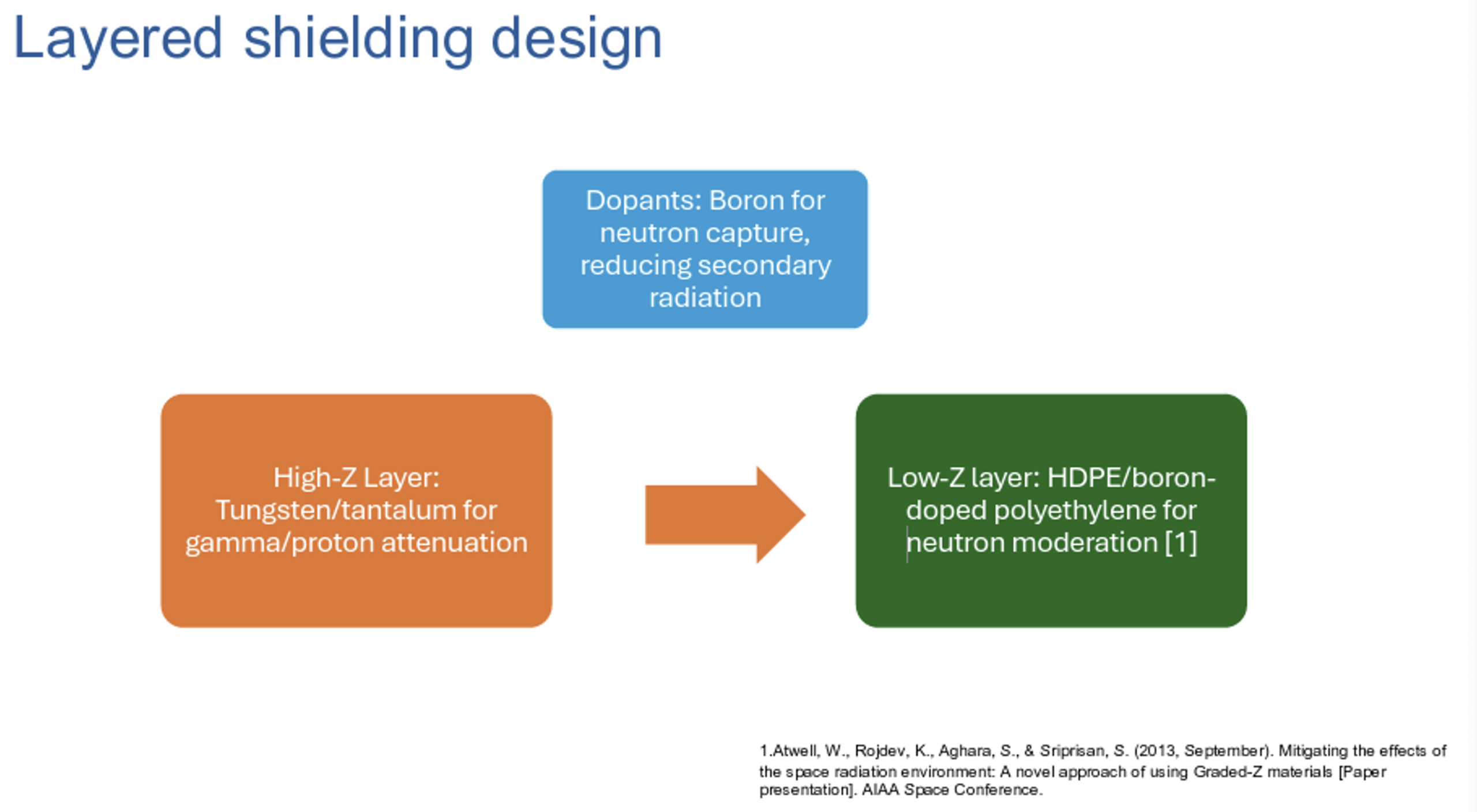
Preliminary results suggest that combining high atomic-number materials (for example, tungsten) to shield gamma radiation with complementary layers containing boron for neutron moderation can reduce the total shielding mass, compared to previously published shield designs.
These findings offer an alternative solution for designing space-capable transceivers that allow for high-speed data transmission at low bit error rates. By evaluating off-the-shelf components for space applications, this research presents a cost-effective option that may help reduce testing costs and accelerate qualification time for new parts, which is greatly needed in the growing space industry today.
Presentation: A testing framework for Microelectronics – Sean Klein, Purdue University
IPv6 war stories
It is commonly thought that ‘enterprise is lagging’ in the world of IPv6 deployment. It was refreshing to see a presentation from a large-scale enterprise provider on their experience in running an IPv6-only enterprise-wide Wi-Fi network. Admittedly in this case it’s a very tech-savvy enterprise, namely Meta. Theirs was a large Wi-Fi deployment:
- With 100,000 wireless clients.
- In 90 cities.
- Served by 28 data centres.
- With 40,000 wireless access points.
- 400 wireless controllers.
- Equipment and associated network management systems sourced from two vendors.
Their rationale was that they were running out of room in the two IPv4 private use prefixes they were using for the corporate network by 2018. The prospect of using an IPv6-only network where each subnet was a complete /64 removed the constant adjustment of subnet assignments across all of their sites to respond to demand growth.
Their migration started with the first vendor’s Wi-Fi equipment, migrating these networks to IPv6-only across 2018 and 2019. Once that was complete, Meta turned their attention to the second vendor’s equipment in 2020.
Wireless Access Points (APs) used DHCPv6 Option 52 to perform controller discovery, which worked as intended. Hosts presented some challenges, as they cannot immediately identify the characteristics of the local network at boot time, and commonly configure their interfaces with both IPv4 and IPv6 addresses as part of the boot process.
The underlying issue is a byproduct of IPv6’s origins in design-by-committee, where multiple solutions to a situation have emerged, and host systems may not support all options. When there are Stateless Auto-address Configuration (SLAAC) and DHCPv6 for stateful assignment from DHCP controllers, issues can arise. Android systems don’t support DHCPv6, while Apple iOS devices use SLAAC as the primary address assignment function and use DHCPv6 for additional information, such as DNS resolver location.
IPv6 makes extensive use of multicast, which can cause problems on large Wi-FI networks, as multicast is handled in the same way as an all-stations broadcast. On Wi-Fi subnets with large client counts, the broadcast traffic loads can be significant. Some effort is made to limit the airtime volume, and neighbour solicitation is performed through the controller rather than by broadcast.
Meta also experimented with the use of DHCP Option 108, which is an instruction from a DHCP server to a client that directs it to disable its IPv4 stack and switch to IPv6-only mode. While this worked on their employee network —where they had greater control over the set of devices and device behaviours — it was a failure on their guest network, where they encountered devices that had already disabled IPv6!
I was struck by one of the conclusions in this presentation, namely that:
Doing IPv6-only for clients is tricky if you don’t have full control over your client base. Even so, we’ve run into weird issues and dependencies, especially when going from one major OS version to another.
And of course, there is the usual source of continuing irritation that is IPv6 fragmentation handling. Meta had to add explicit ACL entries to permit the passing of IMCPv6 Packet Too Big messages and IPv6 packets with the IP Packet Fragmentation Extension Header.
Presentation: Large Scale Enterprise WiFi using IPv6 – Steve Tam, Meta
IPv4 war stories
These days, most recent IPv4 deployments in the public Internet rely on Network Address Translation (NAT). In most parts of the Internet there is still sufficient residual IPv4 use in the online provision of goods and services to rule out an IPv6-only offering.
As a piece of shared infrastructure, NATs work most efficiently when they are large. A single NAT, working with a single pool of IPv4 addresses will operate more efficiently than a collection of NATs with the address pool divided up between them.
Large-scale networks bring the internal client traffic into a large-scale NAT cluster. You can’t just locate NATs at the physical exterior portals of your network. You need to create bidirectional internal paths between customers and the NAT cluster, and bidirectional paths from the exterior portals to the same NAT cluster.
Simple destination-based hop-by-hop routing frameworks find this challenging and we have resorted to a more complex overlay that has its own terminology. These frameworks include Pseudowire Headends (PWHE) with Policy-Based Routing (PBR), and Virtual Routing and Forwarding (VRF) router configurations to segregate traffic streams into distinct routing contexts.
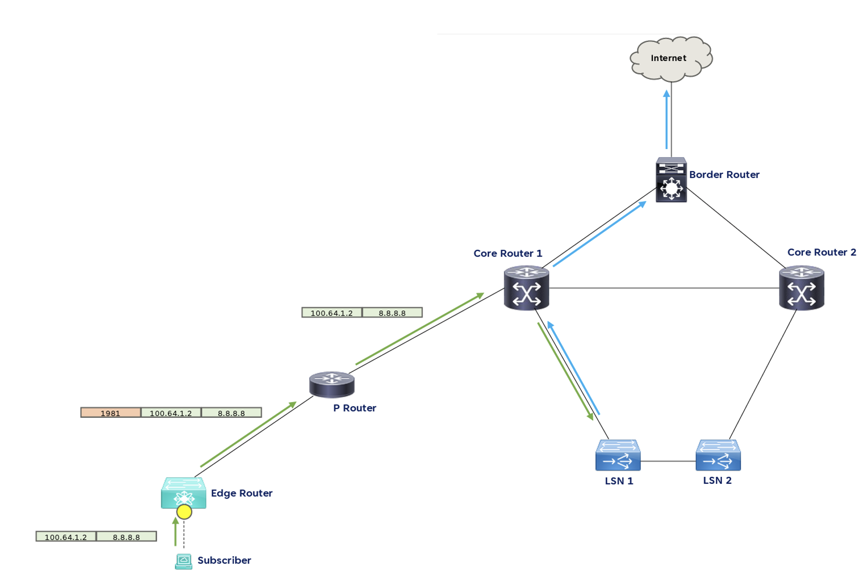
This presentation explored a different approach to this challenge, using Segment Routing (SR). The carrier NATs are directly connected to the internal core routers, and these routers form a single segment using a shared anycast loopback. PBR in the core routers allows outbound traffic from clients to be directed to the internal NAT, while translated outbound traffic from the NAT — using the same destination address — is directed to the network’s border router. Inbound traffic is similarly directed from the border router to the NAT cluster.
Personally, I’m not sure if swapping the complexity of VRF for the complexity of SR makes the scenario any less complex.
Presentation: Large Scale NAT Routing To Centralized Cluster over SR – Renee Santiago, Ezee Fibre
High performance SSH
The Secure Shell application, SSH, has a well-deserved reputation for being slow. It delivers an authenticated and secured access channel, which today is highly desirable, and it’s highly available on many platforms. But, it can be slow to the point of being actively discouraged! Why should adding encryption to a transport channel exact such a hefty performance penalty?
SSH is slow because it has a maximum application layer receive buffer size of 2MB. This makes the effective window of a SSH connection the minimum of this 2MB buffer and the underlying TCP connection. SSHv2 is a multiplexed protocol where a single underlying TCP connection carries multiple simultaneous data channels, with each channel using its own flow control.
SFTP has additional flow controls imposed on top of the SSH control. The effective receive buffer for an SSH file transfer is the minimum of these three limits. The maximum performance is limited to one effective receive buffer per Round-Trip Time (RTT). The result is that in small RTT networks, SSH performs well, but this drops off as the RTT increases.
Chris improved SSH performance by resizing the internal SSH buffers to the same size as the TCP buffers. Encryption is not a significant performance penalty, so lifting the receive buffer size in SSH lifts the performance of the protocol to a speed that’s comparable to TCP on the same network path.
HPN-SSH extends OpenSSH by lifting the receive buffer size, using parallelized cipher operation, and adding session resumption with SCP. It’s compatible with any SSHv2 client or server implementation. The SSH bottleneck is on the receiver, not the sender, so an HPN-SSH client extracts greater performance from an existing SSH server.
His approach uses a call to the underlying TCP socket to return its TCP window size, and then uses this value to force the SSH channel buffer to grow to the same value. This value is sent to the sender as receive-available space, which directs the sender to send this amount of data inside a single RTT.
It might sound simple, but Chris observed that he has been working in this for 20 years, and it’s more complicated than it might initially appear. The OpenSSH call graph is reproduced from Chris’ presentation — it’s complicated!
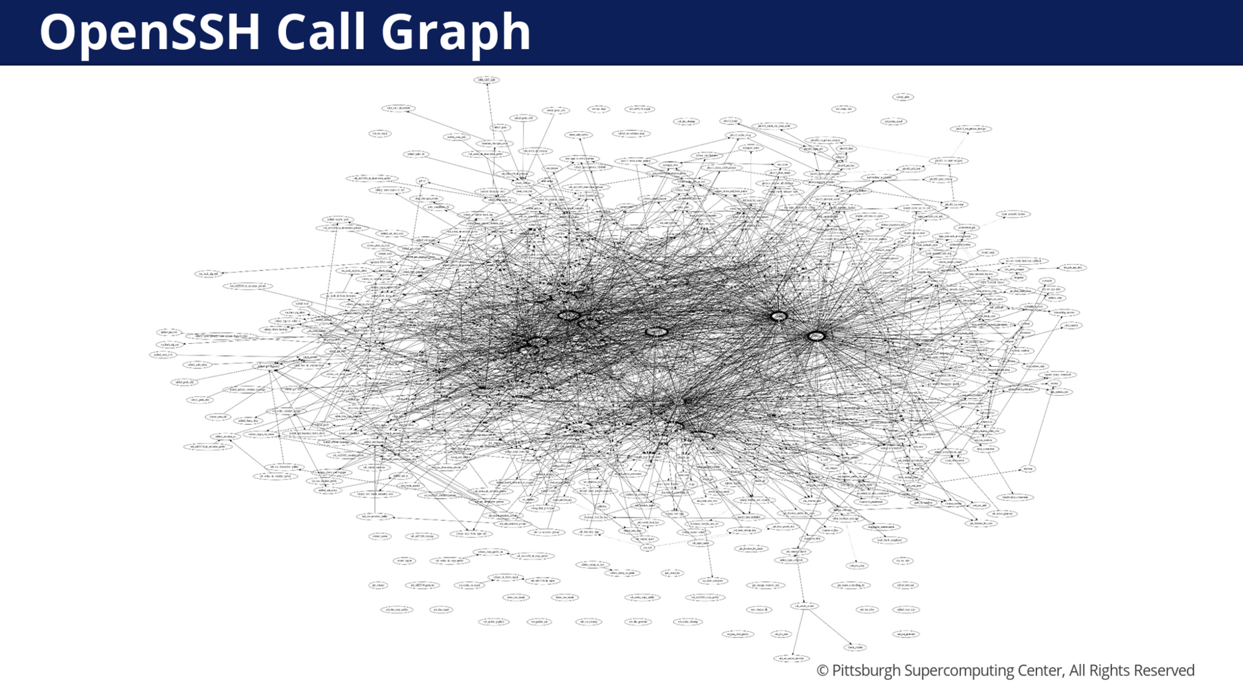
After removing the receive buffer bottleneck, other bottlenecks are exposed. Ciphers are processed in a serial manner, completing each SSH datagram before moving on to the next. Parallelizing ciphers is a lot more challenging than it sounds in OpenSSH, as the cipher implementations are highly customized. Translating these ciphers to a threaded implementation is a significant exercise. Their approach was to extract the ‘raw keystream’ data into distinct data caches, and then perform the Exclusive Or (XOR) function with the data blocks in parallel. This has dramatically improved the performance of HPN-SSH.
There is also the question of whether authentication and channel encryption need to go together. Yes, encryption is needed to secure authentication, but for non-sensitive data the data transfer then shifts to a NONE cipher, which can achieve higher data transfer performance. They are also working on MultiPath-TCP as a runtime option, which can allow for network roaming and parallel path use.
In the quest for higher speed, it appears that it’s more stable to use a collection of individual streams working in parallel. For example, a single 10Gpbs transfer is less stable than 10 parallel 1Gbps transfers. They have developed a tool to run on top of HPN-SSH, parsyncfp2, a parallelized version of the rsync tool, that will achieve more than 20Gbps sustained over a high-capacity high-speed infrastructure.
Presentation: HPN-SSH – Chris Rapier, Pittsburgh Supercomputing Centre
From the archives
The US telephone system of the mid-1980s is a great example of large-scale design by committee and the complexities that follow. The AT&T monopoly, which had been established in 1913 with the Kingsbury Commitment, came to a partial end in 1984. The single company was broken up into nine Regional Bell Operating Companies and a single long-distance carrier.
Central to the breakup was the concept of a Local Access and Transport Area (LATA). These are geographic areas where phone calls between parties are managed by the Local Exchange Carrier (LEC) as either a local call or a regional toll call. LATAs translated to the phone number address plan, where the initial digit designated the LATA.
The US State system also intruded into this structure. There were various forms of call types, each with its own tariff and each with its own body providing oversight. There were calls within the same LATA and same State with oversight from the State’s Public Utilities Commission (PUC). There were calls within the same LATA but between different States, with oversight from the Federal Communications Commission (FCC). There were calls between LATAs, but within the same State, which were handled by the long distance Inter Exchange Carrier (IXC), with oversight by the PUC. Calls between LATAs across State boundaries were handled by an IXC with oversight from the FCC.
The system had many built-in anomalies. The State PUCs were often a less effective market regulator than the FCC, leading to some long-distance intra-State calls costing more than inter-State calls. This system of local monopolies in the LATAs by the LECs was opened to competition with the Telecommunications Act of 1996, which introduced the Competitive Local Exchange Carrier (CLEC).
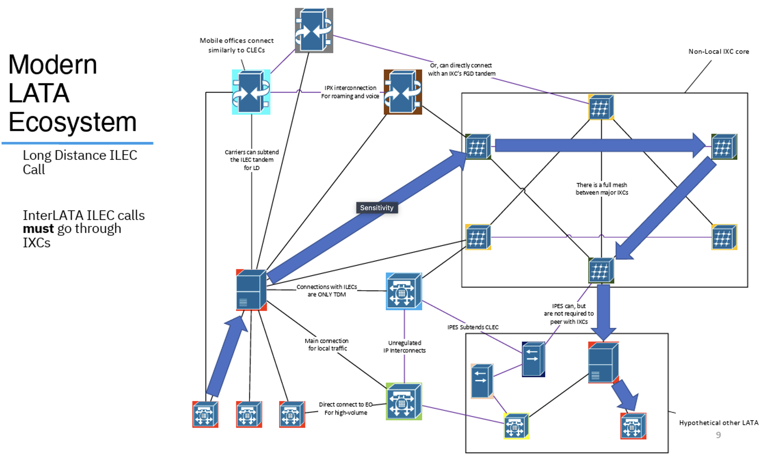
In the world of conventional telephony, based on Time Division Multiplexing, interconnects between carrier networks were the subject of regulatory constraint. It was mandatory for an ILEC — one of the ‘original’ LECS — to interconnect with a CLEC upon request. However, within the ILEC, CLEC and IXC structure call routing is also highly constrained, and LECs must use an IXC when the call is made across LATAs (Figure 7).
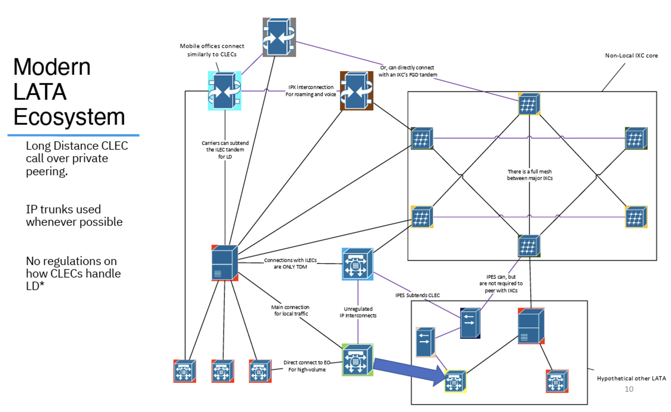
The IP network has had a profound effect on the public switched telephone network (PSTN) in the US. Not just in the technologies that carry voice over IP networks and switching calls, but in this structure of CLECs and IXCs. There are no regulations about how CLECs handle long distance calls using IP carriage, so the same long distance call can be routed directly between CLECs using IP interconnection (Figure 8).
When you add number portability to the mix, the phone number address plan has to carry the burden. A phone number needs to be mapped to a Local Routing Number (LRN), which is a call routing number code used in path call establishment though the mess of LECS, CLECS and IXCs.
The database containing these LRNs is operated manually, like a collection of CSV files that are loaded into switches to guide call routing. On the Internet an update in BGP propagates across the entire network in an average of 70 seconds. A new number block entry in the LRN table takes some 60 days to take effect!
That all this works at all is a miracle!
Presentation: Journey to the Centre of the PSTN – Enzo Damato
From the future
Much has been said about so-called quantum computers in recent years. Quantum physics encompasses the concept of wave/particle duality and replaces determinism with probabilistic functions that contain random elements, including the role of an observer and uncertainty, superposition, interference and entanglement.
Classical physics describes the behaviour of the physical universe at a large scale, while quantum physics describes this behaviour at atomic and subatomic scales. Quantum-scale objects exist in multiple states at the same time as a probabilistic wave, termed a superposition. These objects will remain in a superposition of probabilistic states until they are measured, at which point the wave function collapses into a definite, classical state.
In quantum computing, the qubit is the fundamental unit of quantum information. It can be implemented by any two-state quantum system, which can be in a state of superposition. Qubits can be entangled with each other, allowing certain calculations to be performed exponentially faster than classical computers.
Two of these calculations, solving discrete logarithms over finite fields and elliptical curves, and factoring large numbers into primes, are important to today’s digital security. The first is used by Diffie-Hellman key exchange and the second is the basis of the RSA cryptosystem. In classical computer terms, it is possible to use key sizes that make computing a ‘solution’ to these problems computationally infeasible. In 1994, Dr Peter Shor devised a quantum algorithm that solves both of these problems in short, finite time on a large-scale quantum computer.
Qubits can be stored as:
- Electron spin.
- Photon polarization.
- Electric current in a superconducting circuit where the current can flow clockwise and counterclockwise at the same time.
- Two hyperfine atomic ground states or trapped ions in a vacuum.
All physical qubit implementations are inherently unstable and noisy, and they are prone to decoherence, where all the quantum information is lost. Quantum noise can be thermal noise, electromagnetic noise and vibration. Like forward error correction codes in classical computing, a logical qubit is a combination of physical qubits using quantum error correction codes, allowing an error in a physical qubit to be corrected by other qubits.
One qubit can represent two states at the same time, two qubits can represent four states, and more generally, n entangled qubits can represent 2n states at the same time. An operation on one entangled qubit instantly adjusts the values of all entangled qubits. The objective is to build quantum computers with a large number of entangled qubits.
Quantum logic gates are components of quantum circuits that perform calculations on qubits by altering the probabilities of measuring a one or a zero and the relative phase between the qubits interfering qwaves. These logic gates are imposed on the qubits by way of different electromagnetic pulses.
Quantum logic gates have high error rates. This limits the circuit depth, which limits algorithm complexity. A quantum algorithm is never run just once, but run many times to produce a probability distribution where the probability of the ‘correct’ answer as a wave probability function is significantly higher than all other possible outcomes.
We’re up to a quantum computer with 24 qubits. It’s going to take a minimum of 2,098 logical qubits to run Shor’s algorithm to break a RSA-2048 key with a stunning 6×10¹⁴ gate operations.
It seems like a truly capable quantum computer is a long time off, but perhaps this is an illusory comfort. In a four-month window at the start of 2025 we saw:
- Microsoft/Atom’s QPU with 24 entangled logical qubits in November 2024.
- Google’s Willow QPU with 105 logical qubits and a 49:1 physical to logical qubit ratio in December 2024.
- Microsoft’s Majorana one QPU with eight error resistant physical qubits that make up eight ‘topological’ logical qubits in February 2025.
- Amazon’s Ocelot QPU with five error resistant, logical ‘cat’ qubits in February 2025.
Authentication is a ‘here and now’ problem. The case to introduce crypto algorithms for authentication that present challenges even to quantum computers — so-called Post-Quantum Cryptography (PQC) — is still not an overwhelmingly strong one today. This includes authenticity in the DNS (DNSSEC) and authenticity in the web (the web Public Key Infrastructure). To play it safe, don’t use extended lifetimes with cryptographic credentials.
Channel encryption is a different matter, and if a definition of ‘secrecy’ includes ‘maintain the integrity of the secret for the next 20 years’, then the likelihood of cryptographically capable quantum computers being available in that period is generally considered to be high. That means that if what you want to say needs to be a secret for the next 20 years, then you need to use PQC right now!
What do you have?
The databases that associate domain names and IP numbers with the names of the entities that control them have had a varied history.
At the outset, we thought it was appropriate to operate a directory, similar to a telephone directory, that allowed a querier to use a domain name, an IP address or an Autonomous System number (ASN). We operated this using a simple query protocol, called whois, where you provided a query (domain name, IP address, ASN), which looked up a registry and returned some details.
whois still works well – it queries the IANA server, who refers it to the relevant RIR database, which returns a block of information relating to the holder of these addresses. For domain names, it’s not working so well because the use of directory proxies to occlude the true domain name holder is extremely common.
But let’s return to number resources and ASNs in particular. While whois does a decent job in returning the registration details for an ASN, can we ask slightly different questions, such as:
- ‘List all the ASNs controlled by an organization?’
- ‘Which other ASNs have been registered by the same organization?’
- ‘Which IP addresses are registered to the same organization that controls this ASN?’
These questions relate to establishing relationships between individual registration entries in the databases operated by the Regional Internet Registries (RIRs). Such relationships are not made explicit in the publicly available registry data, either in responses to individual whois queries, or by processing the daily database snapshots published by the RIRs.
However, if you:
- Take these database snapshots — which contain organization names.
- Combine this data with entries contained in the Peering Database.
- Use these organization names as search keys to web crawlers.
- Pass this through some LLM model to distill out the organization name.
You can then construct your own organizational entity relationship as an overlay to the RIR database. A research group at Virginia Tech has done exactly this with the tool asint.
There is little doubt that the key to securing funding for your research program these days is to use the key terms ‘AI’ or ‘Quantum’, or preferably both, in your research proposal. Alternatively, there are simpler approaches.
The relationship between resource holders and the resources they control is available in the RIRs’ data records. There is an item of public information that can lead you straight to the answer without a hint of AI! It’s the daily extended stats file published by the Number Resource Organization.
As the file description indicates, column eight of this report:
is an in-series identifier which uniquely identifies a single organization, an Internet number resource holder. All records in the file with the same opaque-id are registered to the same resource holder.
Never underestimate the awesome power of grep. To list all the IP number resources used by APNIC Labs I can start with ASN 131072 and use that to find all the Labs’ address resources as follows:
$ curl https://ftp.ripe.net/pub/stats/ripencc/nro-stats/latest/nro-delegated-stats >stats

$ grep `egrep "asn\|131072" nro-stats | cut -d '|' -f 8` stats

apnic|AU|asn|9838|1|20100203|assigned|A91872ED|e-stats

apnic|AU|asn|24021|1|20080326|assigned|A91872ED|e-stats

apnic|JP|asn|38610|1|20070716|assigned|A91872ED|e-stats

apnic|AU|asn|131072|1|20070117|assigned|A91872ED|e-stats

apnic|AU|asn|131074|1|20070115|assigned|A91872ED|e-stats

apnic|AU|ipv4|1.0.0.0|256|20110811|assigned|A91872ED|e-stats

apnic|AU|ipv4|1.1.1.0|256|20110811|assigned|A91872ED|e-stats

apnic|AU|ipv4|103.0.0.0|65536|20110405|assigned|A91872ED|e-stats

apnic|AU|ipv4|103.10.232.0|256|20110803|assigned|A91872ED|e-stats

apnic|AU|ipv4|203.10.60.0|1024|19941118|assigned|A91872ED|e-stats

apnic|JP|ipv4|203.133.248.0|1024|20070522|assigned|A91872ED|e-stats

apnic|AU|ipv4|203.147.108.0|512|20080326|assigned|A91872ED|e-stats

apnic|AU|ipv6|2401:2000::|32|20070619|assigned|A91872ED|e-stats

apnic|AU|ipv6|2401:2001::|32|20110803|assigned|A91872ED|e-stats

apnic|AU|ipv6|2408:2000::|24|20191106|assigned|A91872ED|e-stats
There! Now that wasn’t so hard, was it?
Presentation: AS-to-Organization Mapping at Internet Scale – Tijay Chung, Virginia Tech
Where are you?
Geolocation on the Internet is somewhat messy. It’s hard enough to locate IP addresses into economies, but when you want to locate into cities, districts, or even street addresses, things get even messier. It’s also useful to ask what the use case of this geolocation information is. Street addresses are fine for a postal network. What a Content Distribution Network (CDN) wants to know is limited to the economy, to figure out if there are applicable content access constraints to apply, and the network-relative distance between the client and the candidate content server points.
As I observed already, the current key to securing funding for your research program these days is to use the key terms ‘AI’ or ‘Quantum’ or preferably both in your research proposal. So, when you have a proposal to use the reverse PTR records in the DNS and apply an LLM to these DNS names, then the research looks even more attractive!
The project presented here applies a form of Machine Learning to associate a host name, as contained in the PTR records of the DNS reverse zone, with a city/state/economy location.
This works quite well! Many network operators embed some structured textual tokens in the DNS names of their equipment, and many then use the same names when populating the reverse space. They can be airport codes, abbreviated city names, suburb names, even street addresses in some cases.
Visit the Aleph project web page to you want to play with their data.
Presentation: Decoding DNS PTR Records with Large Language Models – Kedar Thiagarajan, Northwestern
Open BGP
These days, we have numerous choices when looking for an open source implementation of a BGP daemon. In addition to their use as routing daemons in open source routers, they are used as route reflectors, looking glasses, routing analysers, Denial Of Service (DOS) mitigators, Software Defined Networking (SDN) controllers and more.
Open source BGP implementations include Quagga, FRRouting, goBGP, Bird, OpenBGPD, RustyBGP, ExaBGP and holo-routing. How ‘good’ are these BGP implementations? What are their strengths and weaknesses? This presentation looked at these eight BGP implementations using a number of criteria relating to their use in an operational environment.
- Quagga was once the major open source BGP tool, but interest in Quagga has waned in recent years and the last commit was eight years ago.
- FRRouting is a fork of Zebra, the BGP component of Quagga, and comes with an active contributor community. Its implementation is on C and Python, and is generally perceived as the successor of Zebra.
- goBGP is a 10-year-old project of BGP implemented in Go, with contributors generally drawn from the Japanese community.
- Bird was developed with support from the Czech CZ.NIC, and has been used extensively for the past 25 years, and is still actively supported.
- OpenBGPD was originally developed for Open BSD, and is still actively supported, with contributors drawn from the German community.
- RustyBGP is a Rust implementation of BGP, originally implemented five years ago. It appears to be stable, in that the last contribution was a couple of years ago.
- ExaBGP is a BGP implementation designed to enable network engineers and developers to interact with BGP networks using simple Python scripts or external programs via a simple API. It appears to be supported with a UK community.
- Holo is another Rust-based BGP implementation.
Admittedly, this exercise can be very subjective, but Claus’ summary of the relative capabilities of these BGP implementations is shown in Figure 9.
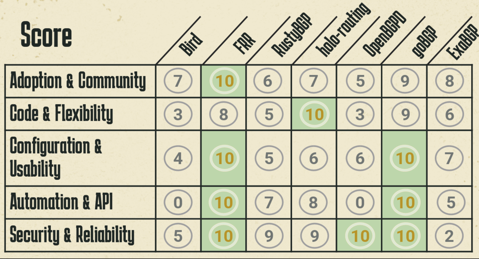
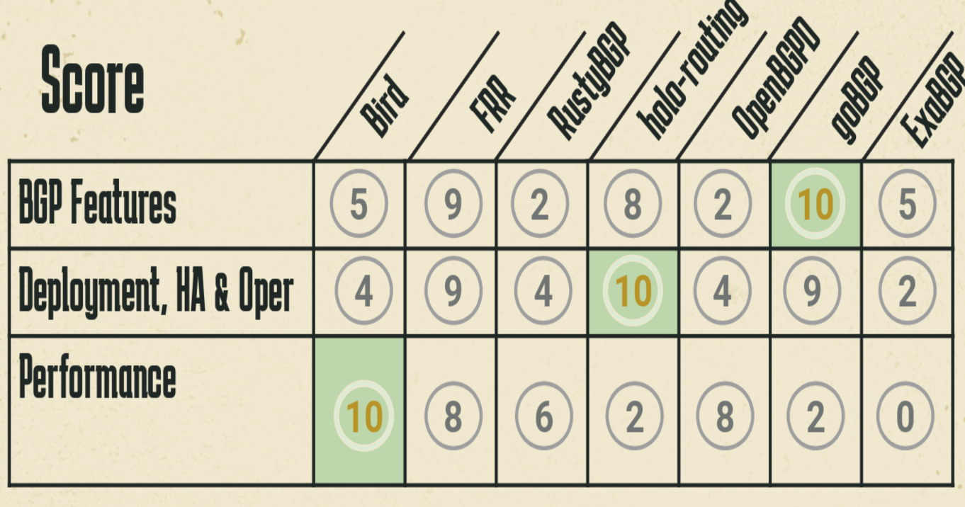
However, these implementations each have different strengths and weaknesses, and a summary of the relative merits of each BGP implementation may be more helpful:
- If you really like working in Python, then ExaBGP is a clear choice.
- If you are looking for an implementation that is fast to load and runs with a small footprint, contains DDoS mitigation measures and supports flowspec, then Bird is a clear choice.
- If you prefer a more conservative option, with easy support and an active community, consider using FRR, GoBGP and Bird.
- If you want use gRPC to inject and collect updates, then its GoBGP and Holo.
- If you want a C implementation, then Bird and OpenBGP are good choices.
- If you are looking to build your own router then FRR, Holo and Bird might make sense for you.
Presentation: Clash of the BGP Titans: Which Open Source Routes It Best? – Claus Rugani Töpke, Telcomanager
NANOG 95
This is a small selection of the material presented at NANOG 95 in October 2025. There were also presentations on ASIC design in high speed routers, Routing security, network measurement tools, and QUIC, among many others.
I had a concern at one point that NANOG had drifted a bit too far into the space of sales and marketing, but I am really pleased to observe that the NANOG Program Committee has done a truly excellent job of turning this perception around. NANOG 95 was a good example of a three-day meeting with valuable and relevant content for almost anyone working in the general areas of network operations and research.
The social contacts you will make at these meetings are every bit as helpful as the content! Yes, it’s a tough call, but I would say that these days it’s among the best network operator meetings on the global calendar!
The views expressed by the authors of this blog are their own and do not necessarily reflect the views of APNIC. Please note a Code of Conduct applies to this blog.
Wow, this is the whole bunch of useful information that tech ppl should study on. Thanks Geoff for the summary.
Geoff – I did the quantum presentation. I wanted to say thank you for summarizing it, adding to it, and distributing it to a wider audience. It’s a big project coming up for all us and I appreciate you spreading the word. Sincerely, Bill.