

Recently, the QUIC Working Group was reviewing an errata for RFC 9002, the description of loss recovery and congestion control for QUIC. There was an error in the description of the algorithm used to compute the variable rttvar, which describes the expected variation of the round-trip time (RTT).
The order of instructions was wrong, leading to underestimating the rttvar by 1/8th. That is, of course, a bug, but the discussion showed that most implementations had already fixed their code.
The discussion also generated quite a few comments on the algorithm itself. It dates from 1988, and it makes hidden hypotheses about the distribution and randomness of RTT measurements, which are wrong, essentially because RTT measurements are very correlated, leading to way more than a 1/8th error.
RFC 9002 describes the loss and congestion control algorithm recommended for QUIC. It includes the computation of RTT and RTTVAR, using the algorithm described in RFC 6298, which is itself copied from the TCP specification updated in 1988 by Van Jacobson:
rttvar_sample = abs(smoothed_rtt - rtt_sample)
rttvar = 3/4 * rttvar + 1/4 * rttvar_sample
smoothed_rtt = 7/8 * smoothed_rtt + 1/8 * rtt_sample
These variables are then used to compute the Retransmission Time Out (RTO in TCP) or the Probe Time Out (PTO in QUIC), using formulas such as:
PTO = smoothed_rtt + max(4*rttvar, timer_granularity) + max_ack_delayThe formulas have two big advantages. They can be computed in a few instructions, which mattered a lot in 1988, and they provide a better evaluation of retransmission delays than the pre-1988 formulas studied by Lixia Zhang in Why TCP Timers don’t work well. But they are making a set of hidden hypotheses:
- The computation of the
smoothed_rttwith an exponential filter of coefficient 1/8 assumes that only the last eight measurements really matter. - The computation of the
rttvarpretty much assumes that successive measurements are statistically independent. - The computation of RTO or PTO assumes that
rttvaris an approximation of the standard deviation of the RTT, and the distribution of RTT can be described by some kind of regular bell curve.
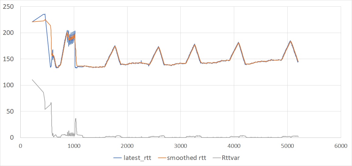
In practice, these hypotheses are not verified. Look for example at Figure 1, showing the evolution of the RTT in a typical QUIC connection. The RTT measurements do not actually follow a random distribution governed by a bell curve. There is a big correlation between successive samples, which causes the rttvar to converge to a very small value.
We also see that the smoothed_rtt variable closely tracks the measurements. In this example, the connection was running at about 75Mbps, the RTT was about 140ms, and there were usually more than 100 packets in flight. The client implementation was sending frequent acknowledgements, which means that the exponential filter was averaging the RTT measurements over a fraction of the RTT.
We also see that the RTT measurements vary mostly with the sending rate of the server. We see a succession of phases:
- The very first measurements during the initial handshake are somewhat higher than average, probably because they incorporate the computing delays caused by the cryptographic processes.
- The RTT measurements then grow quickly during the “slow start” ramp-up, until the server acquires an estimate of the connection bandwidth.
- In the next period, the server follows the BBR algorithm, which periodically probes for a higher bandwidth, with each probe resulting in a slight increase of the RTT.
If the server was using Reno, the third phase would exhibit a ‘saw tooth’ pattern caused by the ‘congestion avoidance’ algorithm. If it was using Cubic, we would see the periodic spikes of the RTT at the end of each Cubic ‘epoch’. But just like with BBR, we would see a high correlation between successive samples. In all these cases, the combination of short-term smoothed_RTT and minimal rttvar is a poor predictor of the next transmission delay.
In the example, there is obviously no competing connection sharing the same path. This is a pretty common occurrence, but there will be connections in which competition happens. Suppose, for example, that a new connection starts with identical characteristics. The new connection will experience high RTTs during its startup phase, and the old connection will also see these higher RTTs. The retransmission timers will not account for such variability, which can easily lead to spurious retransmissions.
I think the timer computation should be fixed to provide robust estimates of the retransmission delays even if acknowledgements are too frequent and RTT samples are correlated. We should also find a way to estimate the maximum plausible delay without making undue hypotheses about the statistical distribution of the delay samples. We should probably replace the current smoothed_rtt and rttvar with a combination of variables, such as:
- A short-term
smoothed_rtt, designed to detect short-term variations of the RTT while smoothing out random variations. See for example the discussion of Hystart and wireless links in this blog post from 2019. - A longer-term version of the
smoothed_RTT, designed to provide an estimate of the average RTT and its variation over several round trips, independently of the rate of acknowledgements. - An estimate of the maximum RTT over the recent past, from which we could derive the retransmission delays.
For this last point, we have to define the period over which the maximum RTT shall be evaluated. Maintaining a maximum since the beginning of the connection is plausible but probably leads to over-estimates for connections of long duration.
Given that the RTT variations are mostly driven by the congestion control algorithm, the number of RTTs over which to compute statistics should probably depend on the algorithm. For BBR, this means covering a complete cycle, including the probing epochs. For Reno, that probably means covering at least a couple of the ‘saw teeth’. For Cubic, probably a couple of epochs. The simple solution could be something like computing a max delay over a rolling series of recent epochs and using that as the RTO or PTO.
Luckily, in most cases, the poor quality of the PTO estimate does not affect QUIC performance too much — most packet losses are detected because further packets were acknowledged first, per section 6.1 of RFC 9002. But having a correct value of the PTO still matters in two cases — if the last packet is an exchange is lost, or if connectivity on a path is lost.
This needs experimenting and collecting results. But first, it means that 35 years after 1988, we should recognize that QUIC timers do not work well.
Christian Huitema (Mastodon) is a researcher and software architect who has written books and developed standards. He’s worked on IPv6, TCP-IP, multimedia transmission over the Internet, security, and privacy. He’s currently working on DNS metrics for ICANN, standardization of QUIC, Picoquic, and privacy and security in the IETF.
Adapted from the original at Private Octopus.
The views expressed by the authors of this blog are their own and do not necessarily reflect the views of APNIC. Please note a Code of Conduct applies to this blog.