

Network design discussions often involve anecdotal evidence, and the arguments for preferring something follow up with ‘We should do X, because at Y place, we did this‘. This is alright in itself as we want to avoid repeating past mistakes in the future. Still, more often than not, it feels like we have memorized the answers, and without reading and understanding the question properly, we want to write down the answer. Ideally, we want to understand the problem and solution space and put that into the current context, discussing various tradeoffs and picking the best solution in the given context. Our best solution for the same problem may change as the context changes. This problem is everywhere. Take a look at this Twitter thread, for example.
Perhaps one solution to this problem is to adopt stochastic thinking and add qualifications while making a case if we don’t have all the facts. The best engineers I have worked with all apply similar thought processes. As world-class poker player Annie Duke points out in Thinking in Bets, even if you start at 90%, your ego will have a much easier time with a reversal than if you have committed to absolute, eternal certainty.
Now we aren’t going to fix human behaviour anytime soon. However, purely from an analytical perspective, for us to be able to quantify things, many times, we need to rely on modelling and simulation. But often, those frameworks don’t exist. One such area was quantifying routing protocol implementation behaviour for a given topology until Sibyl arrived to help us. At a high level, Sibyl proposes various metrics to measure routing protocol implementation, allows you to spin up the topology of a given size with a given protocol implementation, and then measures those metrics for a given failure.
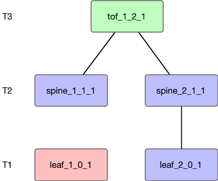
Sample topology
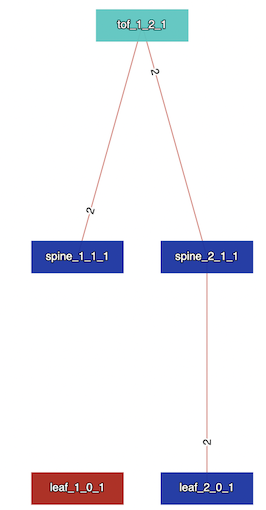
We will start with the most basic topology to understand various metrics for a convergence event using node failure as a trigger event. In Figure 1, we have a simple three-level fat-tree with a radix of 2. We will use Free Range Routing (FFR) based eBGP for routing. One thing to note is that Sibyl refers to T3 switches as the top of the fabric (ToF). For the type of failure test, we will assume node failure and fail leaf_1_0_1.
As shown in Figure 1, the routing stack is FRR. One behaviour to remember with FRR/eBGP is that an eBGP neighbor advertises routes back to the neighbor from whom it learned, which will eventually get rejected due to the AS-PATH loop. This is important because it impacts the number of packets getting injected as part of a convergence event.
For example, if we have three routers R1 – R2 – R3 using eBGP peering, you can see in the below output how R2 is advertising the R1 learned route back to R1. When R1 stops advertising its 10.0.0.1/32 to R2, we will see two BGP withdraws between R1 – R2. R1 will send one BGP withdrawal to R2, and R2 will send a BGP withdrawal to R1. If you are curious about why that behaviour is, refer to this thread.
### R2 has eBGP session to R1 and R3.

R2# show ip bgp summary

Neighbor        V         AS   MsgRcvd   MsgSent   TblVer  InQ OutQ  Up/Down State/PfxRcd   PfxSnt Desc
R1(eth1)        4      65000        62        61        0    0    0 00:02:21            1        3 R1
R3(eth2)        4      65002        62        61        0    0    0 00:02:21            1        3 R3

### R2 has 10.0.0.1/32 from R1 in the BGP RIB.
R2# show ip bgp

   Network          Next Hop            Metric LocPrf Weight Path
*> 10.0.0.1/32      10.1.0.1(R1)             0             0 65000 i
*> 10.0.0.2/32      0.0.0.0(R2)              0         32768 i
*> 10.0.0.3/32      10.1.0.6(R3)             0             0 65002 i

### R2 is receiving 10.0.0.1/32 from R1
R2# show ip bgp neighbors 10.1.0.1 received-routes

   Network          Next Hop            Metric LocPrf Weight Path
*> 10.0.0.1/32      10.1.0.1                 0             0 65000 i
*> 10.0.0.2/32      10.1.0.1                               0 65000 65001 i
*> 10.0.0.3/32      10.1.0.1                               0 65000 65001 65002 i

### R2 is advertising 10.0.0.1/32 back to R1
R2# show ip bgp neighbors 10.1.0.1 advertised-routes

   Network          Next Hop            Metric LocPrf Weight Path
*> 10.0.0.1/32      0.0.0.0                                0 65000 i
*> 10.0.0.2/32      0.0.0.0                  0         32768 i
*> 10.0.0.3/32      0.0.0.0                                0 65002 I
If we look at the BGP events at R3, When the prefix is unreachable on R1, R3 receives a withdrawal from R2 and then sends another withdrawal back to R2.
Withdraw received:
2022-12-28 20:35:21.329 [DEBG] bgpd: [PAPP6-VDAWM] eth1(R2) rcvd UPDATE about 10.0.0.1/32 IPv4 unicast -- withdrawnWithdraw sent:
2022-12-28 20:35:21.380 [DEBG] bgpd: [WHJ94-YXNE1] u1:s1 send UPDATE 10.0.0.1/32 IPv4 unicast -- unreachable
2022-12-28 20:35:21.380 [DEBG] bgpd: [G259R-NCBEJ] u1:s1 send UPDATE (withdraw) len 28 numpfx 1
2022-12-28 20:35:21.380 [DEBG] bgpd: [QYC2K-N0CET] u2:s2 send MP_UNREACH for afi/safi IPv6/unicast
Framework methodology
The Sibyl methodology includes failure and recovery tests. Failure tests include common faults like a node or link failure and measure how a routing protocol implementation reacts to those failures. For a given test, it verifies that the fabric has converged, measures the messaging load induced as part of the event, the blast radius (locality) of the messaging load, and the number of rounds it took for the implementation to converge.
The framework avoids time synchronization issues by using a logical clock and only counts the relevant Protocol Data Unit (PDU) to the event.
Metrics
Messaging load
Sibyl measures the messaging load by counting the number of packets originated by a test and computes the aggregate size. In our example, when a Network Layer Reachability Information (NLRI) is withdrawn as part of the leaf failure, we will see 2 withdraws between each eBGP adjacency, resulting in an aggregate packet count of six (messaging load). We can use this to observe how the messaging load increases as the topology size increases. This will also allow us to compare routing protocols for how the messaging load differs on a given topology.
Locality (blast radius)
Sibyl measures the blast radius of a failure or recovery event by applying the following steps:
- For each link of the network, the number of packets received by the interfaces of that link is computed. Only relevant PDUs that were triggered as part of the event are counted.
- Compute the topological distance of the links from the event (basically, how far away the link is from the event). If an event is like a node failure, all the links attached to the node have a topological distance of 0.
- Then you combine the above 2 in a vector L[i] where i represents the topological distance = 0,1,2, .. n and L[i] represents the number of packets received by the link at that topological distance.
- A scalar value representing a metric for blast radius can be computed, which is a sum of the product of L[i]∗(i+1). This inherently gives more weight to values with higher topological distance.
We can use this to measure the blast radius impact for a routing protocol and see how it changes as the topology grows.
In our example, each link observes 2 withdraws. This gives us a blast radius score of 12.
| Topography distance | 1 | 2 | 3 |
| Packets injected | 2 | 2 | 2 |
State rounds
One problem with just counting aggregate packet counts is that it doesn’t provide insight into how much back and forth happens as part of the convergence event. State rounds try to capture these waves of packets transmitted as part of a convergence event. First, it builds a node-state timeline — a timeline of packets sent or received by each node during the failure event. An arrow represents the packets being sent from one node to another node.
Below is the node-state timeline for our topology. The horizontal axis is the timeline, the vertical axis is the fabric nodes, and the arrows represent the packets being sent from one node to another.
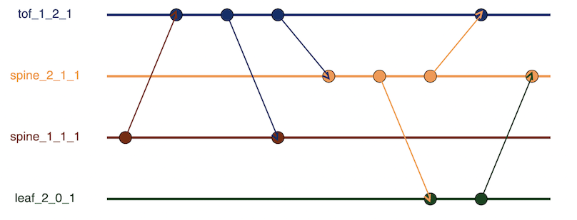
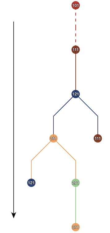
Figure 3’s node-state timeline builds a node-state graph G, in which the edge captures how the nodes transition between states. In the node-state timeline, we can see how Node 111 (spine_1_1_1) sends the packet to tof_1_2_1, which then sends the withdrawal back to spine_1_1_1.
This is also represented in the node-state graph (Figure 4). From the node-state graph, we can count the maximum number of edges, which is four. This tells us that the convergence event takes four rounds to complete. This is fascinating as graph depth gives us a metric for the number of waves it takes for a protocol in a given topology to converge. The number of vertices in the graph indicates the overall amount of state changes induced by an event.
I think this is super useful as we can measure flooding events in topology, the impact of any flooding improvements claimed by a protocol, compare various protocols and see how noisy they are, and so on.
Protocol comparisons
Now, let’s do some comparisons. We will use the following fat-tree topology sizes: (2,2,1), (2,2,2), (3,3,1),(3,3,3),(4,4,1) and (4,4,2) with FRR implementations of BGP, IS-IS, and Openfabric. A single-leaf device is used for the failure test. We should expect OpenFabric to perform better than vanilla IS-IS due to the flooding optimization it contains.
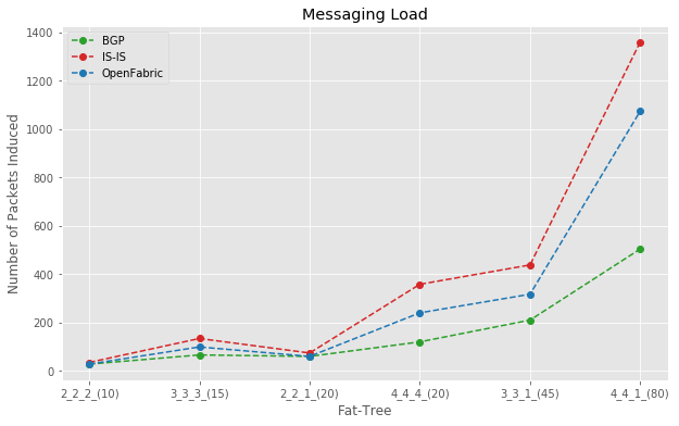
Messaging load comparison
Figure 5 shows the messaging load (the number of packets induced) due to single-leaf device failure. The X-axis contains the fat-tree type and the number of nodes in that fat-tree. For example, a 2_2_2_(10) is a fat-tree with 10 nodes. It is expected that the messaging load will increase as the size of the fat-tree grows, but you can see how that differs among various protocols.
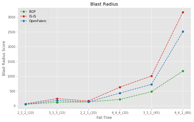
Blast radius comparison
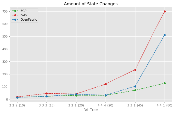
Amount of state change comparison
The below plot shows the total number of state changes observed as part of a failure event. This is the total number of vertexes in the Node-State graph.
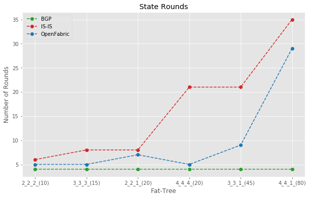
State rounds comparison
Figure 8 measures how many cycles of waves and backwashes happened before the network converged. BGP held fairly steady in this regard, while IS-IS and Openfabric were chatty.
Closing thoughts
We looked at how Sibyl introduces metrics that establish measures for comparing routing protocol implementation on fat-trees and allow us to compare various routing protocol implementations. This post only looked at how FRR’s BGP, IS-IS, and Openfabric behave for a few fat-tree topologies. But this can be generalized for comparing any vendor’s implementation or expanded to not compare implementation behaviour on composite topologies, which may be a collection of fat-trees.
I want to thank Tommaso Caiazzi, for helping me sort out some initial glitches with Sibyl, and many thanks to him and the team for creating Sibyl.
Diptanshu Singh is a Network Engineer with extensive experience designing, implementing and operating large and complex customer networks.
Adapted from the original post on Diptanshu’s blog.
The views expressed by the authors of this blog are their own and do not necessarily reflect the views of APNIC. Please note a Code of Conduct applies to this blog.