Storing and retrieving IP prefixes efficiently

Storing and searching a full table of IP prefixes from the default free zone appears to be a solved problem, since this is the bread and butter of BGP-speaking routers. Several research and engineering efforts have gone into making longest-matching prefix searches for IP addresses in routers happen at wire-speed.

Our goals are a bit different though. We don’t require the fastest searches as modest performance will do in this area. But we do have additional wants, like modest memory consumption, decent write performance, and so on.

Why do we want this?

Eventually, we want to build an engine for BGP that’s open source, modular and focuses on analytics. Seen from a distance, this looks very much like a Routing Information Base (RIB) stored in a router somewhere. The biggest differences would be that we store way more data linked to each prefix and would like to query our data in ways other than just by IP address or prefix. We strongly believe the Rust programming language is best situated to help us do this, and you’ll find that all example implementations mentioned in this blog post are written in Rust.

So, let’s summarize our wish list:

• As we just saw, we need to analyse a full table of IPv4 (currently around 900,000 unique prefixes) and IPv6 (currently somewhere over 100,000 prefixes)
• We want to store data accompanying these prefixes of arbitrary type and size
• We want this metadata to be retrievable by IP address or IP prefix, but we also want to be able to aggregate on prefix, prefix ranges, time, and so on
• We need to be able to retrieve more/less specifics of prefixes with reasonable performance
• We need to read and write to this data structure frequently, simultaneously from and to different streams
• It needs to handle bursts of BGP messages from each of these streams
• We need to be able to store the state at any time, preferably to different kinds of storage backends (in-memory data structures, disk, messaging system)
• And, finally, it needs to be able to run on commodity (server) hardware and mainstream server operating systems (most probably a Linux distribution), so we can leave our bag of tricks with TCAMs, FPGAs, AVX-512 and so forth at the doorstep

Of donkeys, mules, and horses

As mentioned in the introduction, there are several research papers available that describe the thoroughbred racehorses among algorithms. A horse can be made to do incredible things, can be incredibly strong, but sadly needs lots and lots of maintenance and special care, proper food, and training. A horse is expensive, both to purchase and maintain.

Then there are donkeys. A donkey can be made to do only a few things successfully, but goes on forever if treated right, needs little food or maintenance. Also, donkeys are cheap. They’re modest, humble animals that’ll work until the day they die.

Or, we could move to using mules, crossbreeds between horses and donkeys. “Mules are reputed to be more patient, hardy and long-lived than horses and are described as less obstinate and more intelligent than donkeys“

In the end, I expect us to crossbreed a mule of our own. But before we start doing so, I’d like you to introduce you to someone else’s fine mule.

A mule — the key-value collection

Let’s start with the mule among data structures, the Associative Array, HashMap, Dictionary, Object. or whatever it’s called in your favourite programming language — basically a collection of (key, value) pairs. Under the hood, they can be quite complex, but for the application programmer they are easy to use. If you don’t know what assumptions to make about the nature of the data and the way you want to interrogate it, aggregate over it, transform it, and so on, such a data structure is your safest bet. It is generally very fast and can be easily stored and retrieved permanently. It is somewhere halfway between a specialized data structure — it only deals with key-value collections — and a generic, all-purpose one, since it has many ways of transforming and searching the data contained in it. A real mule, in my opinion.

Let’s consider a full table of IPv4 data. To simulate a full table, I’ve downloaded a RIS whois file from ripe.net, which holds a list of prefixes with their originating Autonomous Systems (AS) and the number of peers of the RIS collector that are seeing this combination of prefix and AS. This resembles the number of prefixes and the topology in a full table in the default free zone.

What we get is something like this:

[
	...,
	"100.4.146.0/24": { "origin_as": 701, ... },
 	"100.4.147.0/24": { "origin_as": 64777, ... },
 	"100.4.147.0/24": { "origin_as": 701, ... },
 	...
]

That’s a cool structure to have. It’s easy to see how we can aggregate data on origin_as, for example. It’s also easy to see how this could be stored as JSON (well, ok, good that you noticed, this actually is JSON, albeit awful). If all you need is to store and retrieve data around isolated prefixes, then you have an answer about what data structure to use.

Matching on a specific prefix (‘exact match’) works really well for the data structure we’ve created so far, but that’s as far as it goes. We can’t even look up an IP address contained in a prefix, since the key is an arbitrary string to the system. One way to get around this is to store the first IP address in the prefix and the last IP address in the prefix into the data structure directly:

[
	"100.4.146.0/24": { 
		"start": 1678021120, 
		"end": 1678021375, 
		"origin_as": 701, ... 
	},
 	"100.4.147.0/24": { 
 		"start": 1678021376,
 		"end": 1678021631,
 		"origin_as": 64777, ...
 	},
 	"100.4.147.0/24": { 
 		"start": 1678021376,
 		"end": 1678021631,
 		"origin_as": 701, ...
  }
]

Now we can iterate over and look for the searched for IP address represented as an integer (more about that later) to fit within the bounds of start and end fields in the data structure. This is as far as we can go on our mule, though. There seems to be no efficient way of keeping track of the relations between IP prefixes with this kind of data structure. Before we go on with our quest for the perfect data structure, let us first examine the precise relationships prefixes can have.

IP prefix hierarchy

The relation of a prefix to other prefixes can be any of three types: a prefix can be less specific than a set of other prefixes, or more specific that a set of prefixes, or neither (disjoint). These relations cannot be efficiently modelled by HashMaps or whatever they are called. We need to get off our mule, do a step back and see if we can find ourselves a donkey. But before we can do that, I first need to tell you about the nature of prefixes.

A prefix is an IP address and a length. An IP address has many representations, but as we already saw, one of these representations is an integer number (a 32-bit integer for IPv4 and 128-bit for IPv6). This integer in its turn represents a fixed series of bits. A prefix can be regarded as the amount of bits in the address part (the part before the slash) indicated by the length part of the prefix. For example, 119.128.0.0/9 boils down to the first 9 bits of the IP address 119.128.0.0/12. Those bits are 0111 0111 1000 0000 0000 0000 0000 0000 and the first 12 bits are 0111 0111 1000, and that’s the whole prefix. Since most computers are bad at storing a sequence of bits with arbitrary length, we’re wasting a few bits by specifying, with the length, how much of the address is what we consider to be part of the prefix, and then we can store the prefix in a fixed number of bits.

Two prefixes share a more/less specific relation if all bits in one prefix are the same as the corresponding bits in the other prefix starting from the left. The smallest prefix with the smallest length is called the less specific and the prefix with the greatest length is called the more specific. If two prefixes do not have all the same bits set, they are called disjoint prefixes. Consider our prefix from the first example as bits 0111 0111 1000. A prefix that looks like this: 0111 0111 1000 0100 111 would be called a more specific of our example, since it shares all the first 12 bits, but it is longer. A prefix 0111 0111 would be a less specific of our prefix. And 1111 0111 1 would be disjoint from our prefix, since the first bit is already different.

Studying this relationship a bit more we can see that there’s a strict hierarchy of relations between prefixes. Each prefix can only have one direct parent that has a prefix length of its own length minus one (yes, yes, except the prefix with length zero, thanks for being pedantic). Each prefix can also only have not more than two descendants with its own length plus one (yes, yes, I know, prefixes with length max length). If we think of each prefix as a node and connect all these nodes together on one side to their parent (if any) and the opposing side to their children (if any), you’ll see that we’re creating a tree! And a specific one at that, a binary tree, which is a tree where each node can only have up to two children.

Now let’s go back to our key-value collection data structure. As we can see, now it will not help us with modelling this tree hierarchy. We can, of course, aggregate parts of our data structure into a temporary structure that models more/less-specifics for a prefix on demand. Doing that, however, would either require scanning all the data structure (if it’s unsorted) and aggregating from there, or scanning parts of the data structure, but then the structure needs to be sorted at all times, and that is a non-trivial task.

If only we could have a data structure next to our beloved key-value structure that keeps the hierarchy…

Comparing donkeys, mules and horses

In order to retain the hierarchical relations between prefixes I’ve made implementations for a binary tree, a radix tree, and a tree bitmap (in two flavours), for the sake of comparison. I’ve tried to keep the implementations as comparable as possible and there are no optimizations applied whatsoever. You can find details about those data structures and their implementations on our website.

Binary trees are the most unassuming of data structures that are cheap and easy to instruct. They are also obstinate, since they cannot be beaten into submission; they just want to do the things they know well and are good at. They’re not known for very efficient memory consumption, but they can be quite speedy! We use the binary tree in a special way, sometimes called a trie.

Radix trees can be considered compressed (binary) trees. Basically, what it tries to do is get rid of nodes in a tree that do not hold information we need. As you may expect, it needs extra machinery to compress and deflate the trees at will and there are bound to be some tradeoffs between speed and memory consumption. As such, a radix tree is a mule, that has some of the simplicity of a straight-forward binary tree and some of the sophistication of a racehorse.

The last data structure I’ve implemented is a tree bitmap, a solid thoroughbred horse. It uses a bitmap, a fancy word for a sequence of bits, to replace swaths of nodes with one structure, to reduce memory consumption.

There are many other data structures out there that are trying to model the hierarchical relations of prefixes, and once again, I’d like to refer you to our website to read all about my considerations for not picking any of those.

I’ve created a few diagrams to show you what these data structures could look like. They all show the same set of prefixes (on the right of each diagram).

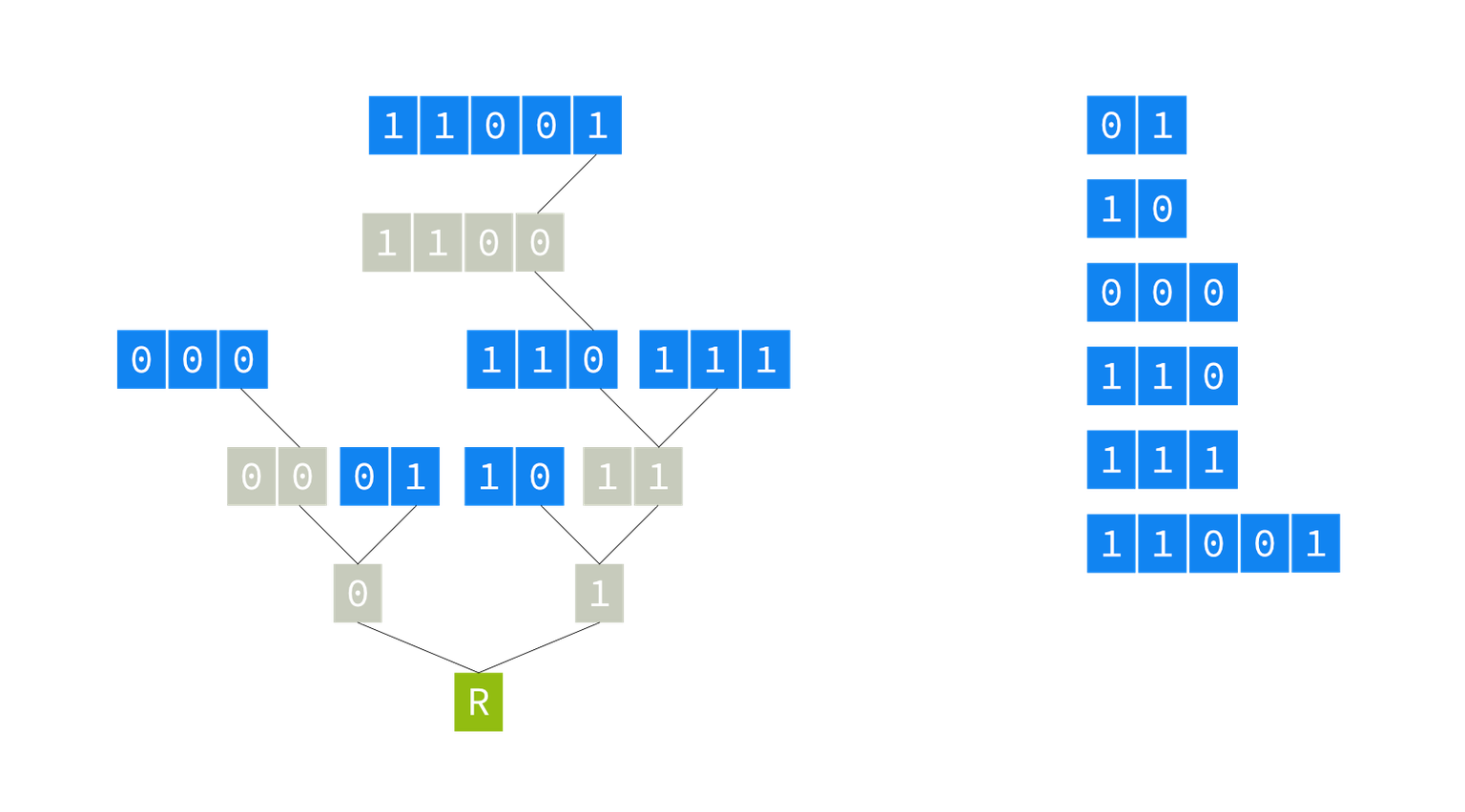
As you can see, we do not only have all the prefixes in their nodes in the tree (the blue nodes), but we also have all intermediary branches and nodes up to the node for that particular prefix. Some of these intermediary nodes are shared with other prefixes; some do not hold any prefix (the grey nodes). So, we must store in the node an indication of whether this node represents a prefix or not. On the other hand, we don’t have to store the prefix identifier itself in the node — the path itself constitutes the identifier for the prefix. In other words, the place in the tree of a node denotes the key of the values it stores inside the node.

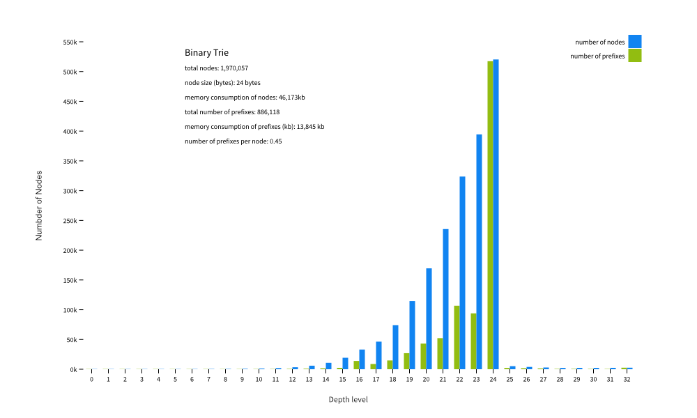
This is a diagram of the distribution of the nodes and prefixes of a full table over the depth of the tree. As you can see, the program created some 2 million nodes for 886,118 unique prefixes, which is an average of 0.45 prefixes per node. One node has a modest size of 24 bytes, so storing all the nodes in memory requires some 48Mb of RAM and 14Mb for the prefixes. The green bars, indicating the number of prefixes in that level of depth in the tree, map directly to the length of the prefixes in the file. Up to /16 you can see the tree is sparse, drops a bit after /16, recovers at /19 and then peaks at /24 (more than half of all prefixes in a full table are of this length) and then almost completely drops off after that.

Building this tree by creating all the nodes takes about 350ms (excluding the loading of the file into memory) on a single thread on a modern CPU. The insert time per prefix is about 390 nanoseconds.

Performing a longest-matching prefix search on a full table tree takes around 26 nanoseconds on average. As an indication of how fast this is, the wire-speed of a 10G Ethernet stream consisting of packets with an MTU of 1,500 is in the order of 1,000 nanoseconds per packet. This is one fast donkey!

Memory consumption isn’t so good, though. It may sound silly to try to compress a memory use of less than 100Mb on modern systems, until you realize that we need multiple copies of this tree in memory in a full-blown analytical engine (one read, one write, one per peer connection, and so on). Also, copying large amounts of memory has a cost that’s probably worse than linear with the amount that’s being copied. So, we want to reduce the memory consumption.

Radix tree

So how can we use less memory? As we already saw, all the 64-bit pointers require lots of memory, as well as slowing down things unnecessarily. It would be great if we could somehow collapse the nodes that are not holding any prefix information, since then we would have fewer pointers, resulting in less memory consumption and less traversal time. This is what a radix tree tries to achieve. Let’s look at our example to see how a radix tree achieves this goal, and why we’ve reverted to using the word tree instead of trie (apart from aesthetics, that is).

I’ve redrawn the prefixes from the previous simple trie example as a radix tree. What’s changed? A number in a small box appeared next to each prefix and two grey nodes disappeared. The idea of a radix tree is that nodes that have only one branch upwards and do not carry a prefix can be eliminated from the tree. Doing so makes a more compact tree. Hopefully, it will also save memory usage. The tradeoff is that we must keep two extra pieces of information at each node.

The first is a number that indicates which bit this node is branching from. The second piece of information that needs to be stored in each node is the IP address part of the prefix of that node.

I made an implementation that tries to be as similar as possible to the simple trie implementation, as shown in Figure 4.

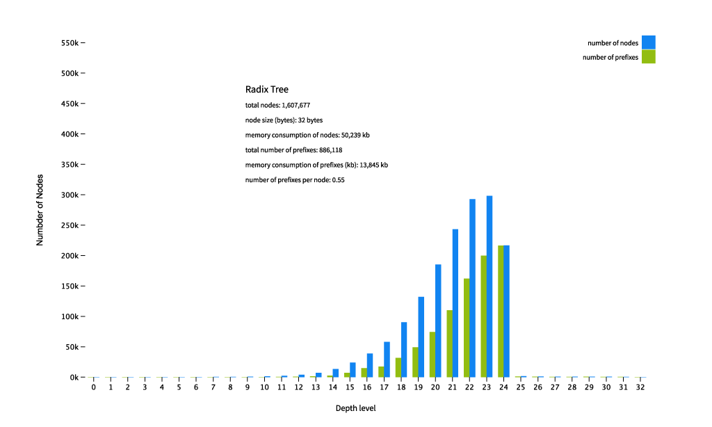
As we can see, the total number of nodes in the radix tree has dropped to some 1.6 million (down from 2 million in a binary trie). The bars are now more evenly spread out over the levels of the tree up until we reach depth 24, and then it drops off. Note that the depth level does not correspond anymore with the length of the prefix: the prefixes are pushed down to fewer deeper levels because of the compression. Insert performance is better than our binary trie as we’re creating fewer pointers, which is costly. Read performance is worse though, which doesn’t matter so much to us, but is unexpected. The idea is that following pointers is a somewhat expensive operation for a CPU, but somehow this pans out differently.

But wait, what? Our memory consumption actually went up! What happened? Our node size has gone up from 24 bytes for a simple binary trie to 32 bytes in our radix trie! Well, remember we had to store the prefix itself in the node? That accounts for the increase of the node size. I used a type that can hold both an IPv6 and an IPv4 prefix, so that requires 8 bytes. The net result is that the reduction in the number of nodes is not weighing up to the increase in node size. We could make an IPv4 and IPv6 specific implementation and then the IPv4 tree could see a reduction in memory consumption when compared to a binary tree. Even then it wouldn’t be too impressive a memory footprint reduction (it would be approximately 45Mb).

It turns out the level of possible compression in a radix tree is heavily dependent on the topology of the uncompressed tree. It basically shines in (very) sparse trees, where several prefixes share the same set of nodes up the tree. As IPv4 full tables grow more and more dense over time, this kind of compression will probably lose most of its benefits. On the other hand, if everybody and their aunt is going to disaggregate (‘deaggregate’) their big prefixes into /24s this compression will pay off better.

A horse — the tree-bitmap

The tree bitmap is quite a different beast. It uses two bitmaps per level in the data structure. A level can hold multiple bits of our prefix at once. It can either store the nodes and prefixes in the data structure itself, or in a completely separate data structure. It is structured in such a way that it tries to be very efficient on memory consumption (memory is slow!) and have the CPU do all of the work as possible (you guessed it, CPUs are fast). Furthermore, it tries to leverage the caching properties of modern CPUs. In other words, a real racehorse. The racing properties are not that interesting to us: we already saw that both our binary tree and radix trie are very fast. What makes it so interesting for us is the ability to store the prefixes and nodes in completely separate data structures.

I’ve implemented two versions of the tree bitmap: one with the nodes and prefixes stored locally inside each node — I’ve named it ‘local-vectors’; and one where we use two global collections and the node only has two collections of indexes into these global collections, dubbed ‘pointer-free’. A vector is an ordered collection of elements, basically a list, hence the name. The last version can be visualized like this:

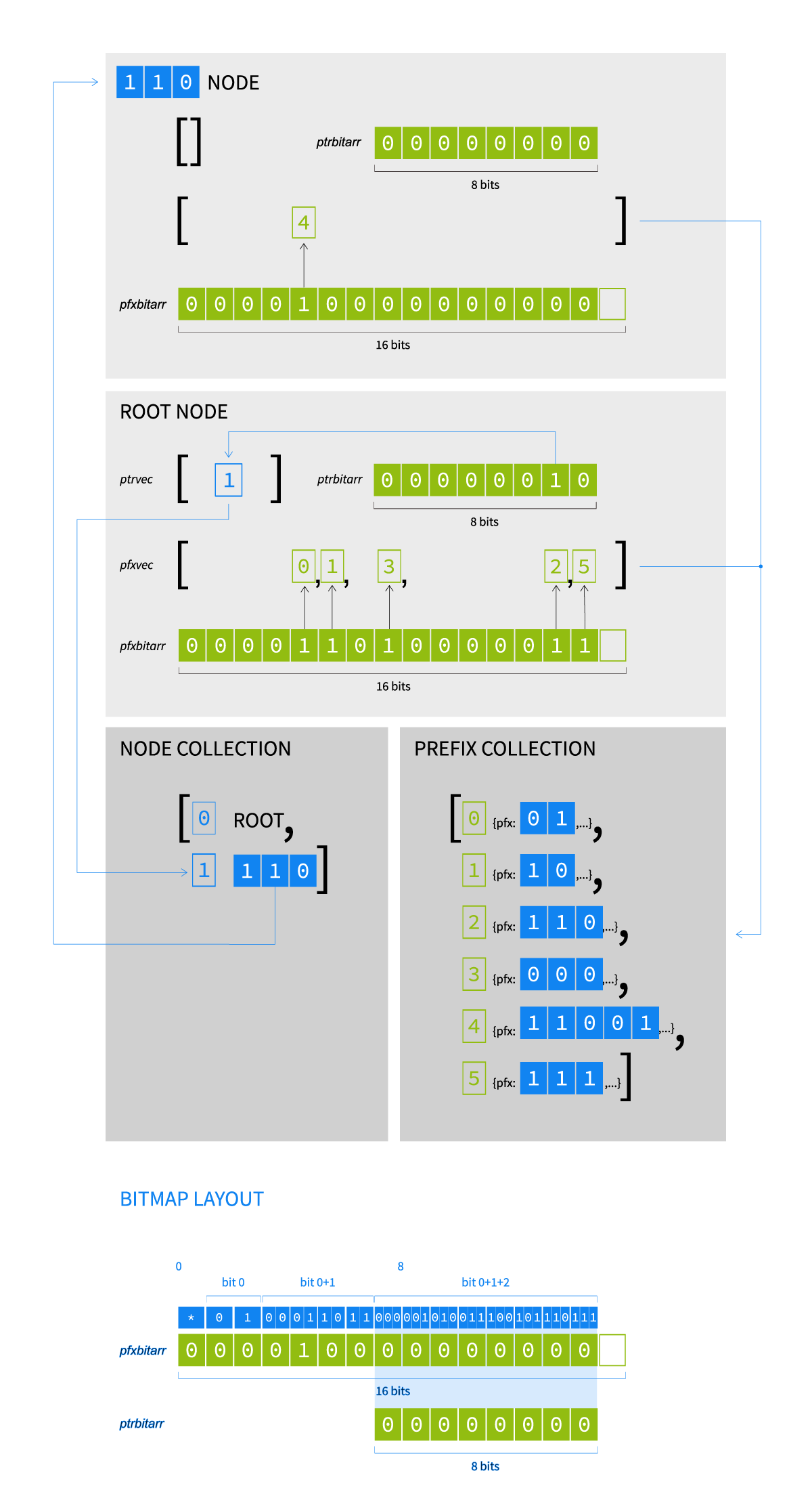
This is an example of a tree bitmap with two nodes, which is necessary to model the same set of prefixes as in the other tree/trie examples.

These are the numbers for some tree bitmaps with different sizes of bitmaps (the numbers within dashes indicate the number of bits that can live on one node).

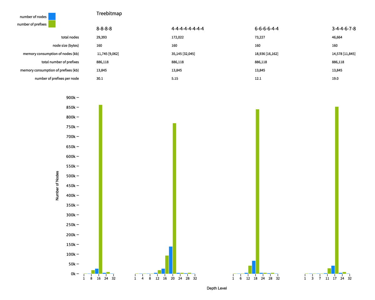
As you can see the number of nodes needed dropped dramatically in comparison with the binary trie and radix tree. Even the variant with the biggest number of nodes, the 4s, features a mere 172,000 nodes. The variant with the smallest number of nodes, the 8s, has only some 30,000 nodes! Even though the nodes are fat in comparison to the other trees — 160 bytes without the vectors inside them — the memory consumption has dropped significantly, ranging from 9Mb for the 4s’ local-vectors (in brackets) to 35Mb for the 4s’ pointer-free.

For read performance, the pointer-free version consistently scores better than the local-vectors version. The pointer-free all-4s even scores better than the radix tree. Reading from two global vectors by index involves following less pointers than jumping to the next node to find its vector. Also, smaller strides perform better than large strides, which may surprise you. Once more I point you to our website for more details about why this happens.

For write performance, the local-vectors version consistently scores better, compared to the pointer-free version with the same strides and by a large margin. Some closer examination reveals the global vectors are reallocating memory for new nodes and prefixes, which takes a significant amount of time.

So, here we see a clear trade-off between memory consumption (the 8s has the lowest) and read/write performance, here the 4s are best. Depending on the storage back-end we may push the needle into a certain direction, for example, if we wanted to persist all nodes and prefixes into a key, value database (on disk or even over the network) then we would care about the number of nodes and prefixes we need to store, so we would choose big stride sizes. If we need to keep up with a very bursty stream of updates we would choose the best write performance and opt for small stride sizes. If we need to create temporary trees — such as for transformations — we could use a local-vectors version tree-bitmap with small stride sizes and so on.

Crossbreeding to full circle

We’ve considered the global data structures up till now to be list-like sorted collections (vectors), where each element in it can be referred to with an index. That’s easy and simple. We can, however, choose any data structure we wanted as long as it can refer to each element in it by a unique identifier and where that unique identifier can be stored inside the nodes. So, if we choose, say, a (key, value) collection as the global data structure, we come full circle!

We started out with a (key, value) collection, went on to try a binary trie, a radix tree and a tree bitmap. Finally, we tried a tree bitmap that features our starting point, the (key, value) collection. We can now enjoy all the advantages of that collection as we saw earlier on, while preserving all the information of the prefix tree hierarchy. There is also the added benefit that an exact-match search could be done directly on the (key, value) data structure instead of going through the tree from the root; data aggregations can be done directly on (a copy of) the (key, value) data structure.

So, this is what we end up with for now: our own crossbreed of donkey and horse, that’s actually closer to horse than I expected. It turned out to be relatively easy to tune the tree-bitmap data structure and its construction algorithm to suit our needs.

Until now, we have only considered our data structures with single-threaded, consecutive reads and writes. In the future, we will take a look at how to take our data structures to the next level and insert, update them, and read from them concurrently. Maybe the pendulum will swing somewhat back to donkey — we’ll see.

How we tested

We loaded a full table 893,943 prefixes in randomized order, performed 2,080,800 consecutive longest matching prefix searches, and ran five runs of each test. Then we took the average of the worst run.

All code can be found in this Github Repository

Jasper den Hertog is a software engineer at NLnet Labs, creating software in Rust, mainly related to routing and RPKI.

This post was adapted from the original at NLnet Labs Blog.

Rate this article

---

The views expressed by the authors of this blog are their own and do not necessarily reflect the views of APNIC. Please note a Code of Conduct applies to this blog.