

TCP congestion control algorithms have continued to evolve for more than 30 years. Much of their success is rooted in the fact that they are loss-based, whereby they use packet loss as the congestion signal. For example, Linux’s default TCP algorithm, Cubic, reduces its congestion window by 30% when encountering packet loss.
There are some cases though, where loss-based TCP algorithms do not work well. For example, in shallow buffers, packet loss might be misinterpreted as network congestion, which results in poor throughput and low network utilization. On the other hand, in deep buffers, it usually takes a long time for the packets to fill up the buffer; this will incur high network delay, which is known as the bufferbloat problem.
To deal with such issues, Google proposed BBR in 2016. Rather than using packet loss as the congestion signal, BBR regulates its traffic based on observed bandwidth and delay values. Specifically, BBR limits its number of packets in flight to be a multiple of the bandwidth-delay product (BDP). Furthermore, BBR also uses pacing to control the inter-packet spacing.
Read: BBR, the new kid on the TCP block
Key points:
- The difference between the bottleneck buffer size and bandwidth-delay product (BDP) typically dictates when BBR performs well. BBR achieves higher goodput under large BDP and shallow buffer size.
- BBR can cause 100x more packet retransmissions than Cubic.
- The unfairness between BBR and Cubic depends on the bottleneck buffer size — with a small buffer size (10KB), BBR can obtain more than 90% of the total bandwidth; with a large buffer size (10MB), Cubic gets around 80% of the total bandwidth.
Motivation for BBR evaluation
Currently, BBR has already been used by the Google Cloud Platform and YouTube servers. However, before adopting BBR, it is important to answer a few questions:
- When is BBR useful (compared to loss-based algorithms, for example, Cubic)?
- What is the downside of ignoring packet losses?
- Is BBR unfair to loss-based algorithms?
My colleagues and I at Stony Brook University conducted an extensive measurement study under different network conditions across different network testbeds (LAN, WAN, Mininet) to do just this. We deployed the traffic controller on the router for fine-grained network parameter control and used Linux Traffic Control (TC) with NetEm to set network delay and Token Bucket Filter (TBF) to set network bandwidth and buffer size.
When is BBR useful?
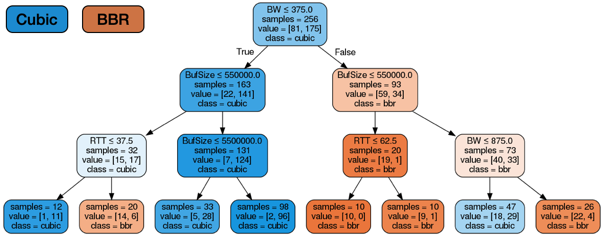
To investigate whether BBR or Cubic achieves higher goodput in different scenarios, we conducted 640 iperf3 experiments in our LAN network. We collected the goodput values of BBR and Cubic during these experiments and generalized the values by a decision tree (using the DecisionTreeClassifier package in Python3) in Figure 1.
In the decision tree, the orange nodes represent instances where BBR achieves higher goodput, whereas the blue nodes represent instances where Cubic achieves higher goodput. We observe in the figure that it is the relative difference between the bottleneck buffer size and BDP that typically dictates when BBR performs well — under small BDP and deep buffer size, Cubic achieves higher goodput, while under large BDP and shallow buffer size, BBR achieves higher goodput.
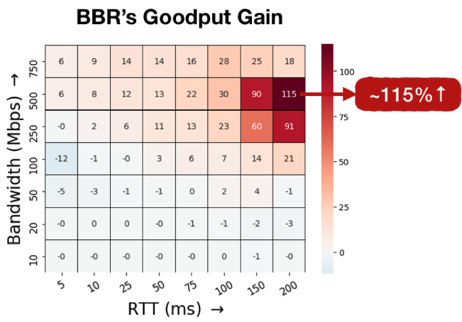
To analyze and quantify BBR’s improvement in goodput compared to Cubic in shallow buffers, we defined the following metric:
GpGain = (goodput|BBR – goodput|Cubic) / goodput|Cubic x 100
For a shallow buffer size (100KB), we show in Figure 2 the heatmap of the GpGain metric under different RTT and bandwidth values. We observed that BBR has significant improvement over Cubic. For example, under 200ms RTT and 500Mbps bandwidth, BBR improves 115% goodput compared to Cubic. This is because BBR uses the bandwidth and delay estimates as the congestion signal rather than packet losses. We will discuss it more next.
What is the downside of ignoring losses?
BBR is designed to keep 2BDP of data in the network (the extra BDP of data is to deal with delayed/aggregated ACKs). As a result, in shallow buffers, the extra BDP of data will cause huge packet retransmissions.
To make things worse, BBR does not treat packet loss as a congestion signal, so the high retransmission maintains over time. The heatmap below (Figure 3) shows the number of packet retransmissions of BBR and Cubic under different RTT and bandwidth values correspondingly.
We observe in Figure 3 that BBR can cause 100x more packet retransmissions than Cubic. This indicates that BBR provides high goodput but at the expense of high packet retransmissions in shallow buffers. Therefore, if the delivered content is sensitive to packet loss, then BBR might not be a good choice. In such cases, the content provider needs to carefully examine the tradeoffs between goodput and quality of experience.
Is BBR unfair to loss-based algorithms?
TCP traffic in the Internet consists of various kinds of TCP flows. Therefore, we need to examine whether BBR is unfair to other TCP algorithms, specifically Linux’s default Cubic.
To this end, we conducted fairness experiments in our Mininet network, where we let two senders generate BBR and Cubic flows to the receiver simultaneously over a 1Gbps link with 20ms delay and different router buffer sizes.
We observe in Figure 4 (left) that the bandwidth share between BBR and Cubic changes for different buffer sizes. Specifically, under small buffer size (10KB), BBR can obtain more than 90% of the total bandwidth. And under large buffer size (10MB), Cubic gets around 80% of the total bandwidth. Therefore, the unfairness between BBR and Cubic depends on the bottleneck buffer size.
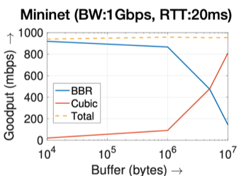
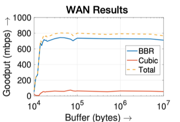
Figure 4 — BBR and Cubic’s bandwidth share under 1Gbps bandwidth, 20ms RTT, and different buffer sizes.
We also conducted the same set of experiments in the WAN network. While we expect the same results, we observe in Figure 4 (right) that the bandwidth share between BBR and Cubic stabilizes as our router buffer size reaches 20KB. This indicates that the bottleneck buffer is in the wild network and out of our control. In practice, we can use this approach to detect the bottleneck buffer in the wild.
BBR’s cliff point
During these experiments we found that there’s a ‘cliff point’ — a loss percentage beyond which BBR’s goodput drops significantly. As we can see in Figure 5 (left), BBR’s goodput maintains at almost full capacity until the loss percentage reaches 20%.
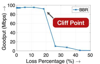
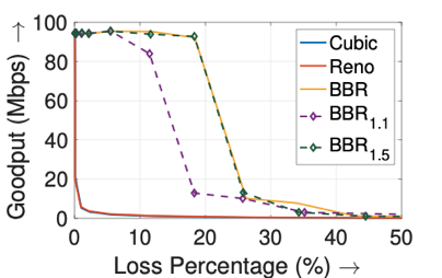
Figure 5 — Goodput vs loss rate (Mininet — 100Mbps bandwidth, 25ms RTT, 10MB buffer). The right graph shows BBR_1.1 (denoting using 1.1 as the maximum pacing_gain), which exhibits a drop at around 9% loss rate, validating our prior cliff point analysis. However, BBR_1.5 exhibits its cliff point much before the predicted 33% loss rate. This is because BBR considers a > 20% loss rate a sign of policing, and so uses the long-term average bandwidth instead of using its maximum bandwidth estimate.
Through our analysis, we found that the cliff point has a close relationship with BBR’s maximum pacing_gain parameter that determines its probing capabilities. If the packet loss probability is p, then during bandwidth probing, BBR paces at pacing_gain × bandwidth (BW). However, due to losses, its effective pacing rate is pacing_gain × BW × (1 − p). Thus, if this value is less than the bandwidth, BBR will not probe for additional capacity, and will infer a lower capacity due to losses.
What is in store for the future of BBR?
Google released BBRv2 a few months ago, which uses both packet losses and ECN to help identify network congestion and achieves better fairness and fewer packet retransmissions than BBRv1.
Although our work focuses on BBRv1, our work reveals that BBR’s performance is sensitive to BBR’s parameter values. Therefore, we envisage that the performance of BBR will be benefited from parameter auto-tuning, rather than using fixed parameter values (as in its current implementation). This would help BBR adapt to various network environments.
This work was presented at IMC 2019 ‘When to use and when not to use BBR: An empirical analysis and evaluation study’
Watch — Yi Cao present ‘When to use and when not to use BBR: An empirical analysis and evaluation study’ at IMC 2019.
Yi Cao is a PhD candidate in the Department of Computer Science at Stony Brook University.
The views expressed by the authors of this blog are their own and do not necessarily reflect the views of APNIC. Please note a Code of Conduct applies to this blog.