BBR, the new kid on the TCP block

The Internet was built using an architectural principle of a simple network and agile edges. The basic approach was to assume that the network is a simple collection of buffered switches and circuits. As packets traverse the network they are effectively passed from switch to switch. The switch selects the next circuit to use to forward the packet closer to its intended destination. If the circuit is busy, the packet will be placed in a queue and processed later, when the circuit is available. If the queue is full, then the packet is discarded.

This network behaviour is not entirely useful if what you want is a reliable data stream to transit through the network. The approach adopted by the IP architecture is to pass the responsibility for managing the data flow, including detecting and repairing packet loss as well as managing the data flow rate, to an end-to-end transport protocol.

In general, we use the Transmission Control Protocol (TCP) for this task. TCP’s intended mode of operation is to pace its data stream such that it is sending data as fast as possible, but not so fast that it continually saturates the buffer queues (causing queuing delay), or loses packets (causing loss detection and retransmission overheads). This desire by TCP to run at an optimal speed is attempting to chart a course between two objectives; firstly, to use all available network carriage resources, and secondly, to share the network resources fairly across all concurrent TCP data flows.

But while TCP might look like a single protocol, that is not the case. TCP is a common transport protocol header format, and all TCP packets use this format and apply the same interpretation to the fields in this protocol header (Figure 1). But behind this is a world of difference. The way TCP manages the data flow rate, and the way in which it detects and reacts to packet loss are in fact open to variation, and over the years there have been many variants of TCP that attempt to optimise TCP in various ways to meet the requirements or limitations that are found in various network environments.

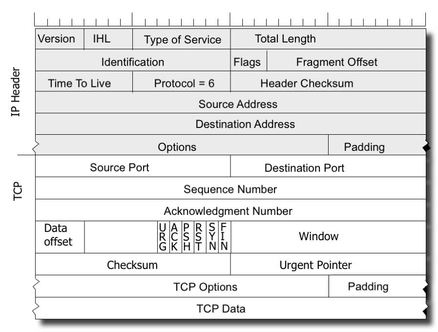
Figure 1 – The Headers for a IPv4 / TCP packet

AIMD and TCP Reno

For many years, the so-called “Reno” flow control algorithm appears to have become the mainstay of TCP data flow control, perhaps due to its release in the 4.3BSD-Reno Unix distribution.

Reno is an instance of an AIMD flow algorithm, denoting “Additive Increase, Multiplicative Decrease”. Briefly, Reno is an “ACK-pacing” flow control protocol, where new data segments are passed into the network based on the rate at which ACK segments, indicating successful arrival of older data segments at the receiver, are received by the data sender. If the data sending rate was exactly paced to the ACK arrival rate, and the available link capacity was not less than this sending rate, then such a TCP flow control protocol would hold a constant sending rate indefinitely (Figure 2).

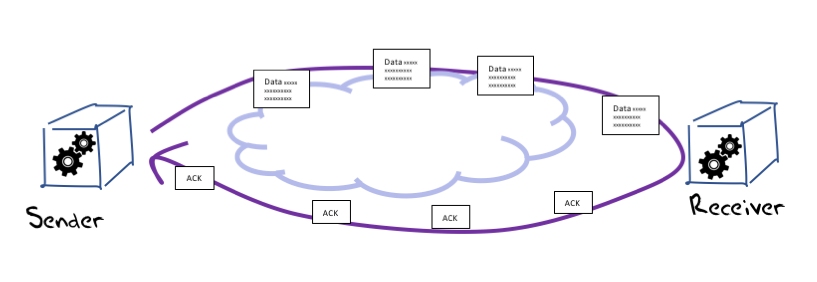
Figure 2 – Ack-pacing flow control

However, Reno does not quite do this. In its steady state (called “Congestion Avoidance”), Reno maintains an estimate of the time to send a packet and receive the corresponding ACK (the “round trip time,” or RTT), and while the ACK stream is showing that no packets are being lost in transit, then Reno will increase the sending rate by one additional segment each RTT interval.

Obviously, such a constantly increasing flow rate is unstable, as the ever-increasing flow rate will saturate the most constrained carriage link, and then the buffers that drive this link will fill with the excess data, with the inevitable consequence of overflow of the line’s packet queue and packet drop. The way TCP signals a dropped packet is by sending an ACK in response to what it sees is an out-of-order packet where the ACK signals the last in-order received data segment. This behaviour ensures that the sender is kept aware of the receiver’s data reception rate, while signalling data loss at the same time.

A Reno sender’s response to this signalled form of data loss is to attempt to repair the data loss and halve its sending rate. Once the loss is repaired, then Reno resumes its former additive increase of the sending rate from this new base rate. The ideal model of behaviour of TCP Reno in congestion avoidance mode is a “sawtooth” pattern, where the sending rate increases linearly over time until the network reaches a packet loss congestion level in the network’s queues, when Reno will repair the loss, halve its sending rate and start all over again (Figure 3).

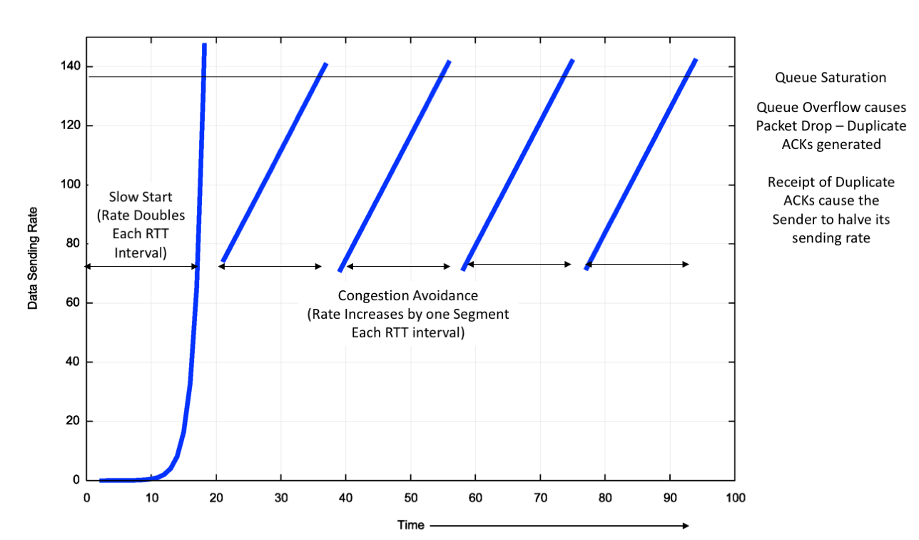
Figure 3 – Ideal TCP Reno Flow Control behaviour

The assumptions behind Reno are that packet loss occurs only because of network congestion, and network congestion is the result of buffer overflow. Reno also assumes that a link’s RTT is stable and the ceiling of available bandwidth is also relatively steady. Reno also makes some assumptions about the size of the network’s queue buffers, in that rate halving will not only stop the queue growing, but it will also allow the buffer to drain.

For this to occur the total packet queue capacity in bytes should be no larger than the delay bandwidth product of the link that is driven by this buffer. Smaller buffers cause Reno to back off to a level that makes inefficient use of the available network capacity. Larger buffers can lead Reno into a “buffer bloat” state, where the buffer never quite drains. The residual queue occupancy time of this constant lower bound of the queue size is a delay overhead imposed on the entire session.

Even when these assumptions hold, Reno has its shortcomings. These are particularly notable in high-speed networks. Increasing the sending rate by one segment per RTT typically adds just 1,500 octets into the data stream per RTT. Now, if we have a 10Gbps circuit over a 30ms RTT network path, then it will take some 3.5 hours to get the TCP session up from 5Gbps flow rate to 10Gbps if the TCP session was accelerating in speed by 1,500 octets each RTT.

During this 3.5-hour period there can be no packet drops, which implies a packet drop rate of less than one in 7.8 billion, or an underlying bit error rate that is lower than 1 in 1014. For an absolutely clear end-to-end channel in an experimental context, this may be feasible, but for conventional situations with cross traffic and transient loads imposed by concurrent flows, this is a completely unrealistic expectation.

As noted above, it’s also the case that Reno performs poorly when the network buffers are larger than the delay bandwidth product of the associated link. And, like any ACK pacing protocol, Reno collapses when ACK signalling is lost, so when Reno encounters a loss condition that strips off the tail of a burst of packets, it will lose its ACK-pacing signal, and Reno has to stop the current data flow and perform a basic restart of the session flow state.

There have been many proposals to improve this TCP behaviour. Many of these proposals make adjustments to the level of increase or decrease per RTT, but stay within the basic behavioural parameters of increasing the sending rate more slowly than its decrease. In other words, these variants all try to be highly reactive to indications of packet loss, while conservative in their efforts to increase the sending rate.

But while it seemed that Reno was the only TCP protocol is use for many years, this changed over time, and thanks to their use as the default flow control protocol in many Linux platforms, CUBIC is now widely used as well, probably even more than Reno.

CUBIC

The base idea was defined with BIC (Binary Increase Congestion Control), a protocol that assumed that the control algorithm was actively searching for a packet sending rate that sat on the threshold of triggering packet loss, and BIC uses a binary chop search algorithm to achieve this efficiently. When BIC performs a window reduction in response to packet drop, it remembers the previous maximum window size, as well as the current window setting.

With each lossless RTT interval, BIC attempts to inflate the congestion window by one half of the difference between the current window size and the previous maximum window size. In this way, BIC quickly attempts to recover from the previous window reduction, and, as BIC approaches the old maximum value, it slows down its window inflation rate, halving its rate of window inflation each RTT.

This is not quite so drastic as it may sound, as BIC also uses a maximum inflation constant to limit the amount of rate change in any single RTT interval. This value is typically larger than the one segment per RTT used by Reno. The resultant behaviour is a hybrid of a linear and a non-linear response, where the initial window inflation after a window reduction is a steep linear increase, but as the window approaches the previous point where packet loss occurred, the rate of window increase slows down. BIC uses the complementary approach to window inflation once the current window size passes the previous loss point. Initially, further window inflation is small, and the window inflation value doubles in size for each RTT, up to a limit value, beyond which the window inflation is once more linear.

BIC can be too aggressive in low-RTT networks and in slower speed situations, leading to a refinement of BIC, namely CUBIC. CUBIC uses a third-order polynomial function to govern the window inflation algorithm, rather than the exponential function used by BIC. The cubic function is a function of the elapsed time since the previous window reduction, rather than BIC’s implicit use of an RTT counter, so that CUBIC can produce fairer outcomes in a situation of multiple flows with different RTTs.

CUBIC also limits the window adjustment in any single RTT interval to a maximum value, so the initial window adjustment after a reduction is linear. This function is more stable when the window size approaches the previous window size. The use of a time interval rather than an RTT counter in the window size adjustment is intended to make CUBIC more sensitive to concurrent TCP sessions, particularly in short-RTT environments.

A theoretical comparison of Reno and CUBIC is shown in Figure 4.

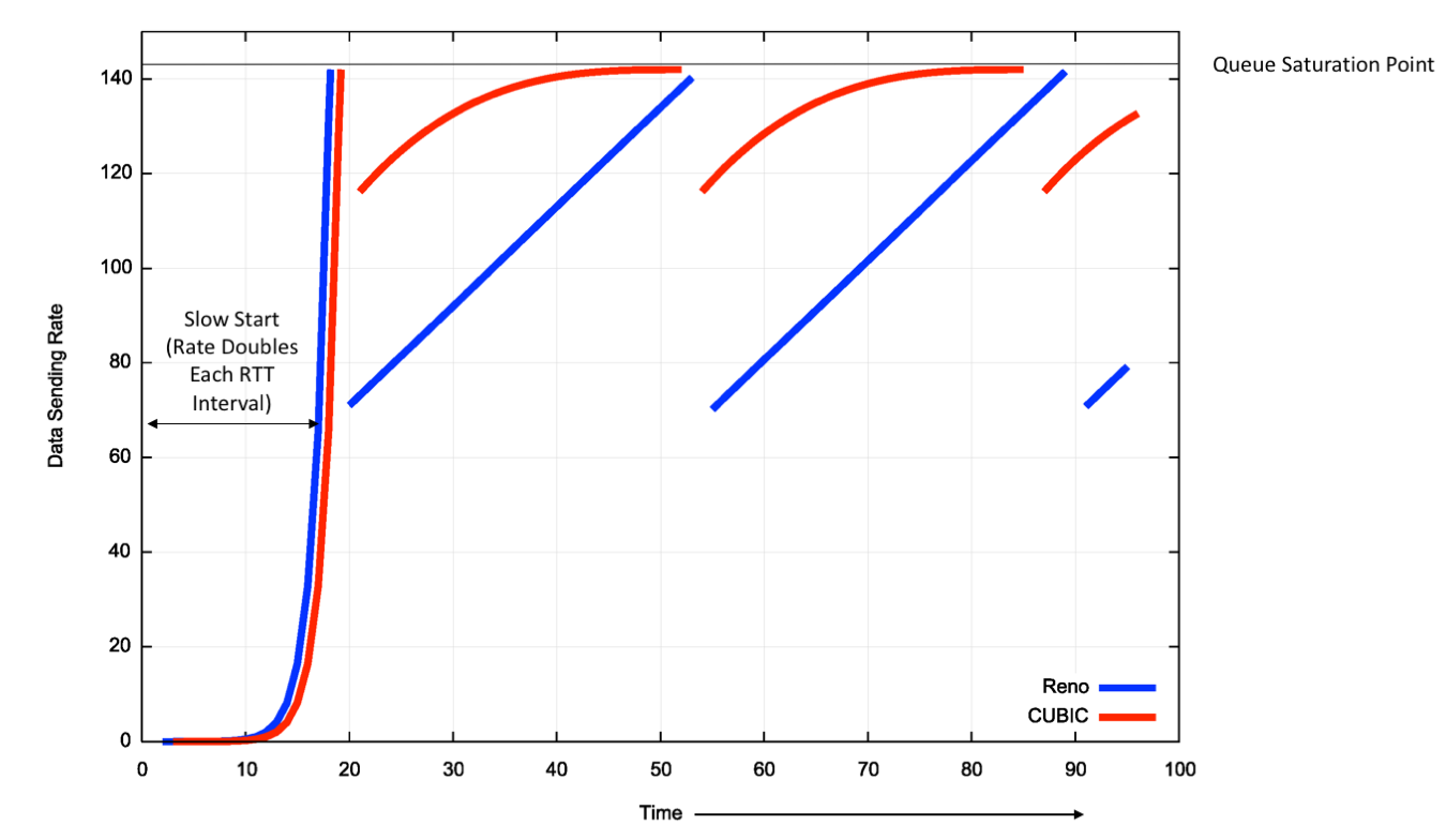
Figure 4 – Comparison of RENO and CUBIC Window Management behaviour

CUBIC is a far more efficient protocol for high speed flows. It’s reaction of packet loss is not as severe as Reno, and it attempts to resume the pre-loss flow rate as quickly as possible. Then, as it nears the point of the previous onset of loss, its adjustments over time are more tentative as it probes into the loss condition.

What CUBIC does appear to do is to operate the flow for as long as possible just below the onset of packet loss. In other words, in a model of a link as a combination of a queue and a transmission element, CUBIC attempts to fill the queue as much as possible for as long as possible with CUBIC traffic, and then back off by a smaller fraction and resume its queue-filling operation. For high-speed links, CUBIC will operate very effectively as it conducts a rapid search upward, and this implies it is well suited for such links.

The common assumption across these flow-managed behaviours is that packet loss is largely caused by network congestion, and congestion avoidance can be achieved by reacting quickly to packet loss.

A Simple Model of Links and Queues

We can gain a better insight into network behaviour by looking at a very simple model of a fixed-sized queue driving a fixed-capacity link, with a single data flow passing through this structure. This data flow encounters three quite distinct link and queue states (Figure 5):

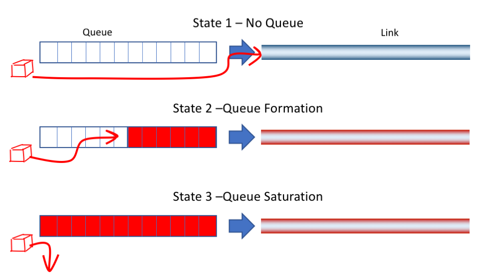
Figure 5 – Queue and Link States

• The first state is where the send rate is lower than the capacity of the link. In this situation, the queue is always empty and arriving flow packets will be passed immediately onto the link as soon as they are received.
• The second state is where the sending rate is greater than the link capacity. In this state, the arriving flow packets are always stored in the queue prior to accessing the link. This is also an unstable state, in that over time the queue will grow by the difference between the flow data rate and the link capacity.
• The third state is where the sending rate is greater than the link capacity and the queue is fully occupied, so the data cannot be stored in the queue for later transmission, and is discarded. Over time the discard rate is the difference between the flow data rate and the link capacity.

What is the optimal state for a data flow?

Intuitively, it seems that we would like to avoid data loss, as this causes retransmission, which lowers the link’s efficiency. We would also like to minimise the end-to-end delay, as ACK pacing control algorithms become less responsive the longer the time between the event causing a condition and the original data sender being notified of the condition through the ACK stream. Simply put, optimality here is to maximise capacity and minimise delay.

If we relate it to the three states described above, the ‘optimal’ point for a TCP session is the onset of buffering, or the state just prior to the transition from the first to the second state. At this point, all the available network transmission capability is being used, while the end-to-end delay is composed entirely of transmission delay without a queue occupancy component.

Reno uses a different target for its TCP flow. Reno’s objective is to keep within the second state, but oscillate across the entire range of the state. Packet drop (state 3) should cause a drop in the sending rate to get the flow to pass through state 2 to state 1 (that is, draining the queue). RTT intervals without packet drop cause the TCP flow to increase the volume of in-flight data, which should drive the TCP flow state through state 2. CUBIC works harder to place the flow at the point of the onset of packet loss, or the transition between states 2 and 3. While this maximises the flow’s ability to place flow pressure of the path, CUBIC does so at a cost of increased delay due to the higher probability of forming standing queue occupancy states.

The question is whether it is possible to devise a TCP flow control algorithm that attempts to sit at that point of optimality that is the onset of the formation of queues, rather than the onset of packet drop.

We can, in theory, tell when this optimal point has been achieved if we take careful note of the RTT measurements of data packets and their corresponding acknowledgements. In the first state, when the sending rate is less than the bottleneck capacity, then the increase in the send rate has no impact on the measured RTT value. In the second state, the additional traffic will be stored in a queue for a period, and this will result in an increase in the measured RTT for this data. The third state is of course identified by packet drop (Figure 6).

The optimal point where the data delivery rate is maximised and the round trip delay is minimised is just at the point of transition from state 1 to state 2, and the onset of queue formation. At this point packets are not being further delayed by queueing, and the delivery rate matches the capacity of the link. What we are after is therefore a TCP flow control algorithm that attempts to position the flow at this point of hovering between states 1 and 2.

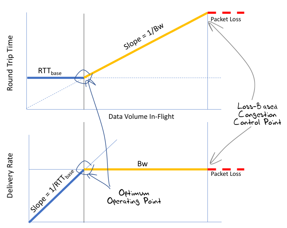
Figure 6 – Delay and Delivery characteristics of a simple Link Model

One of the earliest efforts to perform this was TCP Vegas.

TCP Vegas

TCP Vegas used careful measurements of the flow’s RTT by recording the time of sent data and matching this against the time of the corresponding received ACK. At its simplest, the Vegas control algorithm was that an increasing RTT, or packet drop, caused Vegas to reduce its packet sending rate, while a steady RTT caused Vegas to increase its sending rate to find the new point where the RTT increased.

TCP Vegas is not without issues. Its flow-adjustment mechanisms are linear over time, so it can take some time for a Vegas session to adjust to large scale changes in the bottleneck bandwidth. It also loses out when attempting to share a link with Reno or similar loss-modulated TCP flow control algorithms.

A loss-moderated TCP sender will not adjust its sending rate until the onset of loss (state 3), while Vegas will commence adjustment at the onset of queuing (state 2). This implies that when a Vegas session starts adjusting its sending rate down, in response to the onset of queuing, any concurrent loss-moderated TCP session will occupy that flow space, causing further signals to the Vegas flow to decrease its sending rate, and so on.

In this scenario, Vegas is effectively “crowded out” of the link. If the path is changed mid-session and the RTT is reduced, then Vegas will see the smaller RTT and adjust successfully. On the other hand, a path change to a longer RTT is interpreted as a queue event and Vegas will erroneously drop its sending rate.

Can we take this delay-sensitive algorithm and do a better job?

BBR

Into this mix comes a more recent TCP delay-controlled TCP flow control algorithm from Google, called BBR.

BBR is very similar to TCP Vegas, in that it is attempting to operate the TCP session at the point of onset of queuing at the path bottleneck. The specific issues being addressed by BBR is that the determination of both the underlying bottleneck available bandwidth and path RTT is influenced by a number of factors in addition to the data being passed through the network for this particular flow, and once BBR has determined its sustainable capacity for the flow, it attempts to actively defend it in order to prevent it from being crowded out by the concurrent operation of conventional AIMD protocols.

Like TCP Vegas, BBR calculates a continuous estimate of the flow’s RTT and the flow’s sustainable bottleneck capacity. The RTT is the minimum of all RTT measurements over some time window that is described as “tens of seconds to minutes”. The bottleneck capacity is the maximum data delivery rate to the receiver, as measured by the correlation of the data stream to the ACK stream, over a sliding time window of the most recent six to 10 RTT intervals. These values of RTT and bottleneck bandwidth are independently managed, in that either can change without necessarily impacting on the other.

For every sent packet, BBR marks whether the data packet is part of a stream or whether the application stream has paused, in which case the data is marked as “application limited”. Importantly, packets to be sent are paced at the estimated bottleneck rate, which is intended to avoid network queuing that would otherwise be encountered when the network performs rate adaptation at the bottleneck point.

The intended operational model here is that the sender is passing packets into the network at a rate that is anticipated not to encounter queuing within the entire path. This is a significant contrast to protocols such as Reno, which tends to send packet bursts at the epoch of the RTT and relies on the network’s queues to perform rate adaptation in the interior of the network if the burst sending rate is higher than the bottleneck capacity.

For every received ACK, the BBR sender checks if the original sent data was application limited. If not, the sender incorporates the calculation of the path RTT and the path bandwidth into the current flow estimates.

The flow adaptation behaviour in BBR differs markedly from TCP Vegas, however. BBR will periodically spend one RTT interval deliberately sending at a rate that is a multiple of the bandwidth delay product of the network path. This multiple is 1.25, so the higher rate is not aggressively so, but enough over an RTT interval to push a fully occupied link into a queueing state.

If the available bottleneck bandwidth has not changed, then the increased sending rate will cause a queue to form at the bottleneck. This will cause the ACK signalling to reveal an increased RTT, but the bottleneck bandwidth estimate should be unaltered. If this is the case, then the sender will subsequently send at a compensating reduced sending rate for an RTT interval, allowing the bottleneck queue to drain. If the available bottleneck bandwidth estimate has increased because of this probe, then the sender will operate according to this new bottleneck bandwidth estimate.

Successive probe operations will continue to increase the sending rate by the same gain factor until the estimated bottleneck bandwidth no longer changes because of these probes. Because this probe gain factor is a multiple of the bandwidth delay product, BBR’s overall adaptation to increased bandwidth on the path is exponential rather than the linear adaptation used by TCP Vegas.

This regular probing of the path to reveal any changes in the path’s characteristics is a technique borrowed from the drop-based flow control algorithms. Informally, the control algorithm is placing increased flow pressure on the path for an RTT interval by raising the data sending rate by a factor of 25% every eight RTT intervals. If this results in a corresponding queueing load, as shown by an increased RTT estimate, then the algorithm will back off to allow the queue to drain and then resume at the steady state, at the level of the estimated path bandwidth and delay characteristics.

There is also the possibility that this increased flow pressure will cause other concurrent flows to back off, and in that case BBR will react quickly to occupy this resource by sending a steady rate of packets equal to the new bottleneck bandwidth estimate.

Session startup is relatively challenging, and the relevant observation here is that on today’s Internet link bandwidths span 12 orders of magnitude, and the startup procedure must rapidly converge to the available bandwidth irrespective of its capacity. With BBR, the sending rate doubles each RTT, which implies that the bottleneck bandwidth is encountered within log₂ RTT intervals. This is similar to the rate doubling used by Reno, but here the end of this phase of the algorithm is within an RTT of the onset of queuing, rather than Reno’s condition of within one RTT of the saturation of the queue and the onset of packet drop.

At the point where the estimated RTT starts to increase, BBR assumes that it now has filled the network queues, so it keeps this bandwidth estimate and drains the network queues by backing off the sending rate by the same gain factor for one RTT. Now the sender has estimates for the RTT and the bottleneck bandwidth, so it also has the link Bandwidth Delay Product (BDP). Once the server has just this quantity of data unacknowledged, then it will resume sending at the estimated bottleneck bandwidth rate.

The overall profile of BBR behaviour, as compared to Reno and CUBIC, is shown in Figure 7.

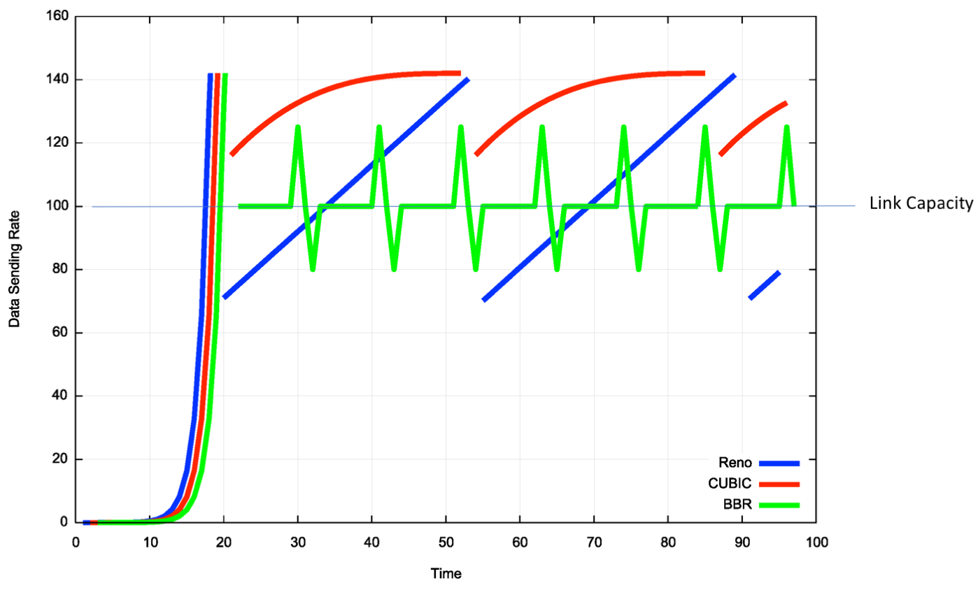
Figure 7 – Comparison of model behaviors of Reno, CUBIC and BBR

Sharing

The noted problem with TCP Vegas was that it ‘ceded’ flow space to concurrent drop-based TCP flow control algorithms. When another session was using the same bottleneck link, then when Vegas backed off its sending rate, the drop-based TCP would in effect occupy the released space. Because drop-based TCP sessions have the bottleneck queue occupied more than half the time, Vegas would continue to drop its sending rate, passing the freed bandwidth to the drop-based TCP session(s).

BBR appears to have been designed to avoid this form of behaviour. The reason BBR will claim its “fair share” is the periodic probing at an elevated sending rate. This behaviour will “push” against the concurrent drop-based TCP sessions and allow BBR to stabilize on its fair share bottleneck bandwidth estimate. However, this works effectively when the internal network buffers are sized according to the delay bandwidth product of the link they are driving.

If the queues are over-provisioned, the BBR probe phase may not create sufficient pressure against the drop-based TCP sessions that occupy the queue and BBR might not be able to make an impact on these sessions, and may risk losing its fair share of the bottleneck bandwidth. On the other hand, there is the distinct risk that if BBR overestimates the RTT it will stabilise at a level that has a permanent queue occupancy. In this case, it may starve the drop-based flow algorithms and crowd them out.

Google report on experiments that show that concurrent BBR and CUBIC flows will approximately equilibrate, with CUBIC obtaining a somewhat greater share of the available resource, but not outrageously so. It points to a reasonable conclusion that BBR can coexist in a RENO/CUBIC TCP world without either losing or completely dominating all other TCP flows.

Our limited experiments to date point to a somewhat different conclusion. The experiment was of the form of a 1:1 test with concurrent single CUBIC and Reno flows passed over a 15.2ms RTT uncongested 10Gbps circuit (Figure 8). CUBIC was started initially, and at the 20-second point a BBR session was started between the same two endpoints. BBR’s initial start algorithm pushes CUBIC back to a point where it appears unable to re-establish a fair share against BBR. This is a somewhat unexpected result, but may be illustrative of an outcome where the internal buffer sizes are far lower than the delay bandwidth product of the bottleneck circuit.

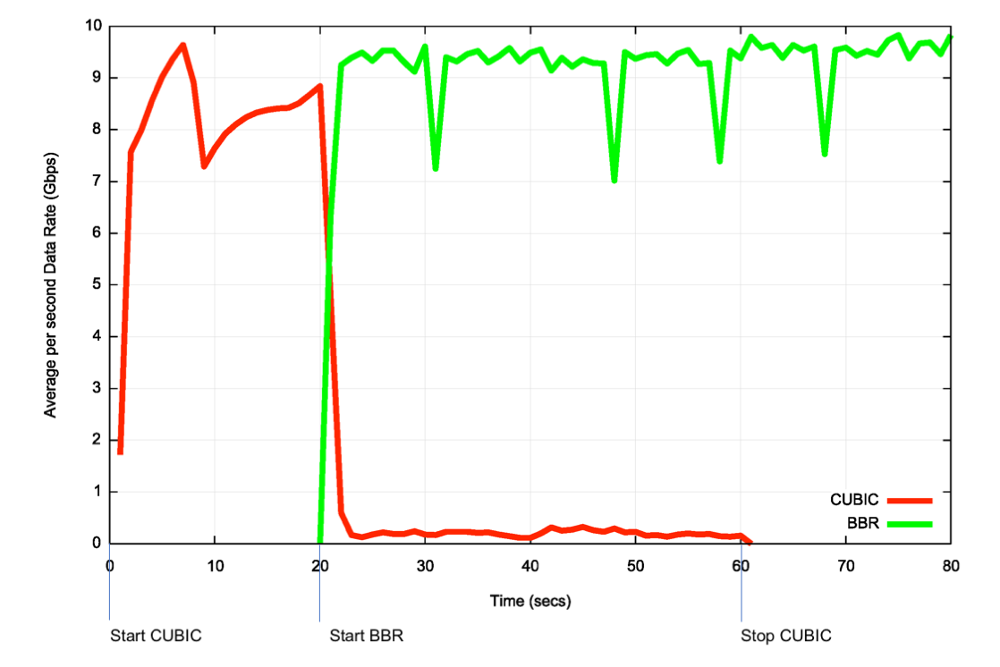
Figure 8 – Test of CUBIC vs BBR

The second experiment used a 298ms RTT path across a large span of the Internet between end nodes located in Germany and Australia. This is a standard Internet path across commercial ISPs, as one would expect to encounter in the Internet. These are not the only two streams that exist on the 16 forward and 21 reverse direction component links in this extended path, so the two TCP sessions are not only vying with each other for network resources on all of these links, but variously competing with cross traffic on each component link. Again, BBR appears to be more successful in claiming path resources, and defending them against other flows for the duration of the BBR session (Figure 9).

Figure 9 – Second Test of CUBIC vs BBR

This is perhaps a less surprising outcome, in that the extended RTT apparently posed some issues for CUBIC, while BBR was able to maintain its path bandwidth estimate in this period. This results point to some level of co-existence between BBR and CUBIC, but the outcome appears be biased to BBR gaining the greater share of the path capacity.

Congestion Control and Active Network Profiling

One other aspect of the Google report is noteworthy:

“Token-bucket policers. BBR’s initial YouTube deployment revealed that most of the world’s ISPs mangle traffic with token-bucket policers. The bucket is typically full at connection startup so BBR learns the underlying network’s BtlBw [bottleneck bandwidth], but once the bucket empties, all packets sent faster than the (much lower than BtlBw) bucket fill rate are dropped. BBR eventually learns this new delivery rate, but the ProbeBW gain cycle results in continuous moderate losses. To minimize the upstream bandwidth waste and application latency increase from these losses, we added policer detection and an explicit policer model to BBR. We are also actively researching better ways to mitigate the policer damage.”

The observation here is that traffic conditioners appear to be prevalent in today’s Internet. The token-bucket policers behave as an average bandwidth filter, but where there are short periods of traffic below an enforced average bandwidth rate, these tokens accumulate as “bandwidth credit” and this credit can be used to allow short-burst traffic equal to the accumulated token count. The “bucket” part of the conditioner enforces a policy that the accumulated bandwidth credit has a fixed upper cap, and no burst in traffic can exceed this capped volume.

The objective here is for the rate control TCP protocol to find the average bandwidth rate that is being enforced by the token-bucket policer, and, if possible, to discover the burst profile being enforced by the traffic conditioner. The feedback that the token-bucket policer impresses onto the flow control algorithm is one where an increase in the amount of data in flight is not necessarily going to generate a response of a greater measured RTT, but instead generate packet drop that is commensurate with the increased volume of data in flight.

This implies that under such conditions a consistent onset of packet loss events when the sending rate exceeds some short-term constant upper bound of the flow rate would reveal the average traffic flow rate being enforced by the token-bucket application point.

Further reading: BBR Congestion Control – Presentation to the IETF Congestion Control Research Group, IETF 97 [1.1 MB] and Google Forum for BBR Development.

Rate this article

Discuss on Hacker News

---

The views expressed by the authors of this blog are their own and do not necessarily reflect the views of APNIC. Please note a Code of Conduct applies to this blog.