BBR evaluation at a large CDN

Bottleneck Bandwidth and Round-trip propagation time (BBR) is a TCP congestion control algorithm that has gained significant market attention due to its ability to deliver higher throughput as reported by many content providers.

In this post, we evaluate BBR (version 1) in the context of Verizon Media’s content delivery network (CDN) workloads, which deliver significant volumes (multiple Tbps) of software updates and streaming video, and quantify the benefits and impact on the traffic. We hope that such an evaluation at a large CDN will help other content providers to choose the right congestion control protocol for their traffic.

What is BBR?

Many content providers and academic researchers have found that BBR provides greater throughput than other protocols. Unlike loss-based congestion control algorithms, such as the ubiquitous TCP-Cubic, BBR has a different operation paradigm; it continuously updates how much data can be in flight based on the minimum RTT the session has seen so far to avoid bufferbloat.

For more information on the operation of BBR, take a look at the original publication from Google here.

Measurement and analysis

To understand the potential for BBR at our CDN, we evaluated BBR at multiple stages, measuring the impact on TCP flows from a few Points of Presence (PoPs).

PoPs represent a concentration of caching servers located in large metro areas. Initially, we performed a small-scale BBR test at a PoP and also performed a full PoP test, with all flows toward clients running BBR.

To identify the benefits that clients would experience, we measured the throughput from our in-house proxying web server logs during the test, as well as socket level analysis.

Metrics to evaluate

Our multi-tenant CDN sees a large variety of client traffic. Many customers have lots of small objects, while others have much larger multi-gigabyte objects. Therefore, it is crucial to identify success metrics that capture actual performance gains across different traffic patterns. In particular, for this evaluation, we identified throughput and TCP flow completion times as the success parameters.

In Figure 1, we show a heat map of common object sizes requested from the CDN versus time taken to serve them. The colour gradient indicates the number of requests in each category. These are representative numbers from a small set of servers, enough to capture the common behaviour only.

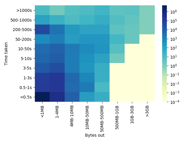
The heat map gives us an understanding of different request patterns. In general, gaining higher throughput is the best indicator of performance gain. However, throughput as a measurement can be very noisy, especially for cases where object size is small (less than a few MBs).

Therefore, based on a separate evaluation of which sizes provide the most reliable assessment of throughput, we use only object sizes greater than 3MB for throughput evaluations. For object sizes less than 3MB, tracking flow completion times is a better metric.

As the first step in our evaluation, we enabled BBR on a few servers at a PoP in Los Angeles and monitored throughput and flow completion times for all the TCP flows. The following results examine a few Internet Service Provider-specific case studies.

A large wireless provider

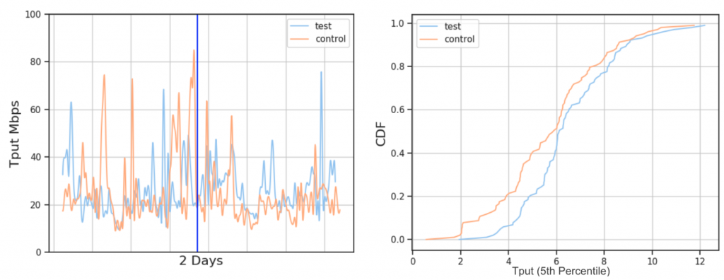
For this wireless provider, as soon as we enabled BBR, on average, we saw a 6-8% throughput improvement. We saw lower TCP flow completion times overall as well. This finding is in agreement with other reports from Spotify, Dropbox, and YouTube, where a clear gain in throughput is seen in wireless networks where packet loss is common, but that is not necessarily an indicator of congestion.

A large wireline provider

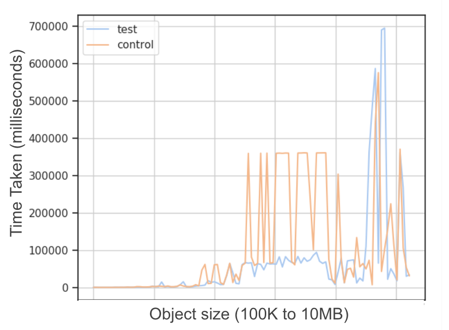
Next, we examined performance for a large wireline provider. Here as well, we saw both throughput (for large objects) and flow completion time (shown in Figure 3) improvements using BBR.

The gains reported from these tests show very promising results for client-side traffic.

Since these gains are on an aggregated view, we decided to dig a little deeper to check if all TCP flows at the PoP saw the benefit of using BBR; or if some TCP flows suffered, and which ones?

At the CDN edge, we performed four different types of TCP sessions:

• PoP-to-Client (as shown above)
• PoP-to-PoP (between data centres)
• Intra-PoP communication (between the caches of the same PoP)
• PoP-to-Origin (PoP to customer origin data centre)

For this study, we considered PoP-to-Client, PoP-PoP, and intra-PoP flows since edge to origin are not as high volume as the other three.

PoP-to-PoP and intra-PoP traffic

It is important to evaluate the impact on these TCP flows as well since in many cases these flows are blockers for client delivery, such as for dynamic content.

For the PoP-to-PoP and intra-PoP traffic throughput, we saw a large regression in performance. Figure 4 shows the impact on intra-PoP and PoP-to-PoP traffic during the same time period:

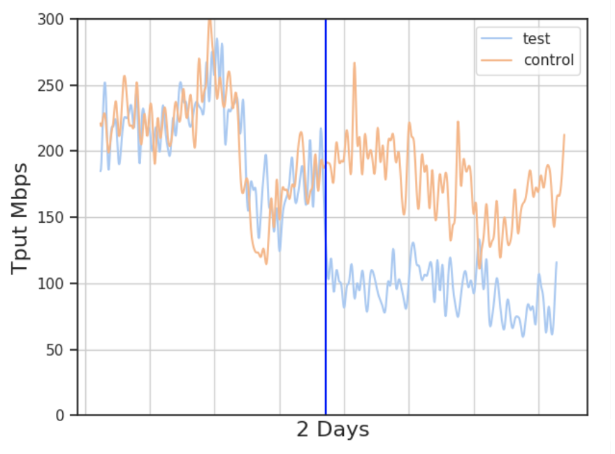
Such clear performance differences between flows to end-users and between data centres have not been reported in previous findings. We need to evaluate why these particular TCP flows suffered; if this is an artefact of hardware or configurations on our CDN; and if so, what tunings would need to be changed.

From further investigation using web server access logs and evaluations from server-side socket data, it appeared that in the presence of both high and low RTT flows, the TCP flows which have very low RTTs suffered from using BBR. We further evaluated cases where less than 0.5KB of data was transferred and found that in most cases, BBR performed similarly to Cubic.

Based on these findings, we concluded that for our traffic patterns, it is better to use Cubic for intra-PoP and PoP-to-PoP communications where RTTs and loss are low. For client-side traffic, it is worth using BBR.

Full PoP test

To evaluate the performance benefit of BBR at a large scale, we ran a full PoP test at a PoP in Rio de Janeiro for all client-facing traffic from our network at that PoP. This PoP made an interesting case study since the location and peering constraints in the region result in higher median RTTs experienced by clients than in other regions.

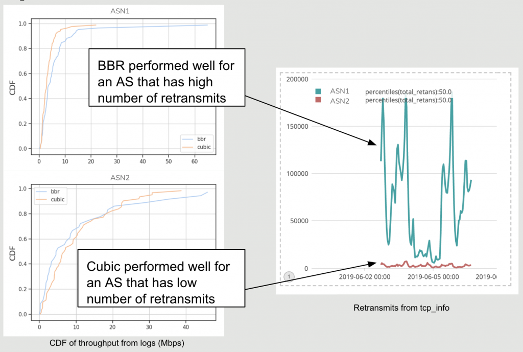
We deployed the change in congestion control algorithm and monitored the performance. A CDF of throughput observed using BBR versus Cubic for the top two ASes (Autonomous Systems) at Rio is shown. As seen in Figure 5, one AS, overall, saw the benefit of BBR while another did not.

To investigate the reasoning behind it, we looked for other TCP metrics collected during the test using the ss utility. A clear distinction is seen in the retransmit rate between these two ASes. Even for ASes with higher RTTs, BBR performs well only for cases that have a high number of retransmits, in other words, for ASes with less loss Cubic has no reason to back-off and performs better than BBR. It is, however, important to note that many of the parameters of TCP Cubic have been carefully tuned on our CDN.

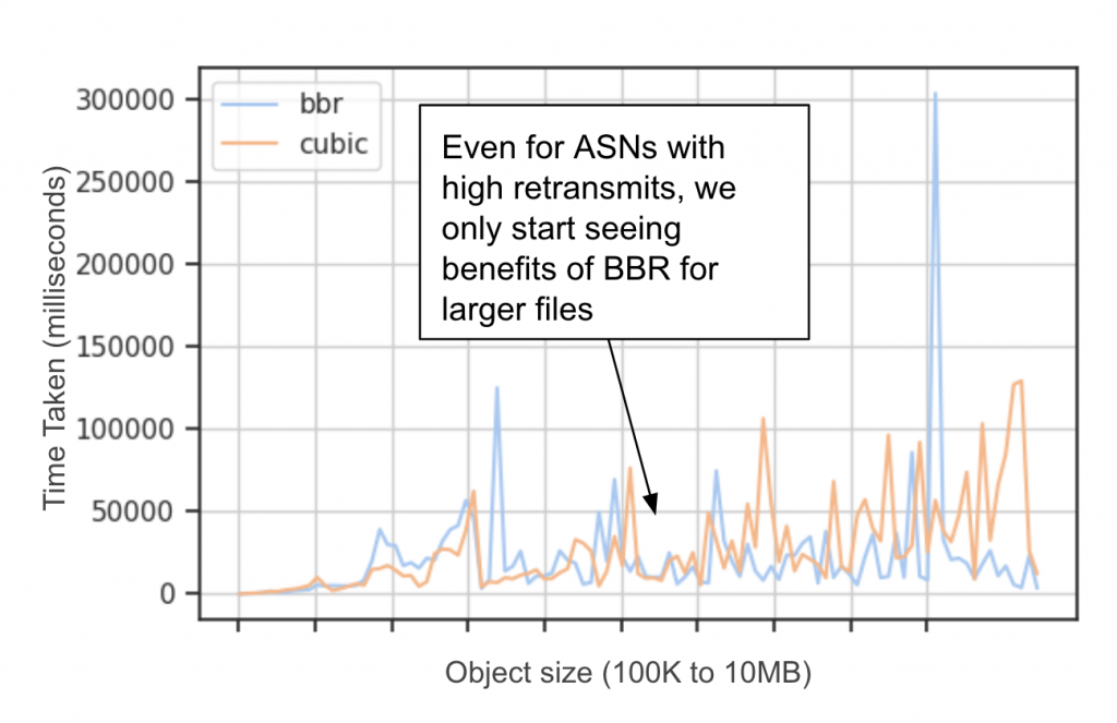
Next, we investigated if all connections from ASN1 shown in Figure 5, showed an improvement in throughput. Figure 6 is a plot of time taken (lower implies better throughput) by BBR and Cubic connections for different object sizes. Here we see that BBR only started showing noticeable benefits for larger objects, in the order of MBs. We did see one anomalous instance using BBR, but could not attribute it to any particular congestion control protocol related issue.

Why does this happen?

There are two dimensions to these results — Cubic vs BBR and BBR vs BBR.

Cubic vs. BBR

BBR is highly reactive to buffer sizes and RTT when it estimates bottleneck bandwidth. In the case of large buffers, where middleboxes might build up a queue, BBR’s estimated RTT increases. Since there is no packet loss, Cubic does not back off in such cases. In other words, PoP-to-PoP style traffic, and therefore Cubic achieves higher throughput. In the case of small buffers, such as wireless clients, the buffer fills rapidly and results in a loss – thus Cubic flows back off, and BBR flows perform better.

BBR vs. BBR

In this scenario, no flow backs off when there is a loss. However, when two flows with different RTT compete for a share of bandwidth, the flow that has higher RTT also has larger minimum RTT and therefore a higher bandwidth-delay product. Thus, that flow increases its inflight data at a much faster rate than the flow that has lower RTT. This leads to reallocation of bandwidth to the flows in descending order of RTT and flows with higher RTTs fill up buffers faster than flows with small RTTs.

Reproducing results in a lab setting

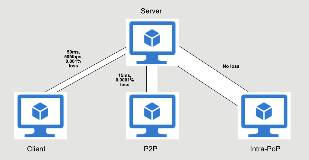
To develop a further understanding of the interactions between flows, we created a testbed environment in Virtual Machines (VMs) that capture behaviour we saw in production. We identified ways to simulate different traffic classes at an edge server as follows:

Client traffic delay was set to ~50ms with losses ranging from 0.001 to 0.1 and bottleneck bandwidth set to 50Mbps. Similarly, for PoP-to-PoP, only loss and delay were set at ~15ms and 0.0001 to 0.01. For intra-PoP traffic, we let the VMs max out available capacity. Finally, simulations were run using various object sizes to capture the multi-tenant nature of our traffic. We ran all three traffic patterns in parallel with an exponential arrival of flows to capture a poisson-style flow arrival distribution. Figure 7 shows the testbed setup.

The goal of this test was to reproduce the issues we saw in the production test, specifically the drop in throughput for small RTT flows for intra-PoP traffic and PoP-to-PoP.

Using this setup, we ran the simulation hundreds of times with simulated background traffic, both Cubic and BBR, and measured ‘time taken’ to complete the flows. The goal of the background traffic is to simulate a production-like environment. Many existing studies focused on running a few flows of Cubic and BBR and evaluating their behaviours. While in those cases it is useful to understand per-flow behaviour, it poorly represents complexities of a large, high-volume CDN. We used client-side flow completion time as a reliable indicator since for small file sizes throughput can be noisy.

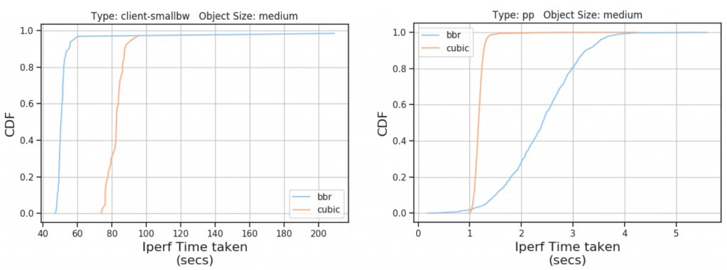
We saw the pattern reappearing in our testbed as well. In Figure 8, we show a CDF of time taken by BBR and Cubic iperf flows in two scenarios: Client traffic and PoP-to-PoP traffic for 3MB (medium size) files. BBR flows fail to catch up to Cubic in a low-loss high-bandwidth setup.

Client traffic (low bandwidth) saw improvement, that is, time taken by BBR flows was less. However, improvement for small files is marginal.

Reproducing these behaviours in the test environment gives us confidence that they are the result of the interaction between different flow types. As a result, any deployment of BBR on the CDN must be aware of the broader impact it may have on a mix of flow types.

BBR flows do not perform well in all scenarios

From our evaluation, we observed that BBR flows do not perform well in all scenarios. Specifically, traffic within a data centre/PoP and traffic among data centres (PoP-to-PoP) suffered when using BBR. In some extreme cases, the throughput was reduced by half. However, we did see a 6-8% improvement in Pop-to-Client traffic throughput.

In this post, we outlined the evaluation of BBR (version 1) in the context of our CDN. We started with a small test of a few servers in a single PoP and evaluated different variables which are of interest to us as a large content provider. In a large scale, full PoP test, we noticed that BBR would help most in cases for ASes where retransmits are high and suggest it is worth using BBR for large files.

Where do we go from here?

If we enable BBR at the system level (all flows), we risk intra-PoP and PoP-to-PoP traffic suffering decreases in throughput.

However, BBR has shown potential and is performing well for client-side traffic. This does motivate us to selectively enable BBR for clients, potentially starting with wireless providers. Moreover, these paths have shallow buffers and wireless loss, an ideal situation for BBR to perform better than other Cubic flows.

We hope that this outline brings some clarity around the use of BBR at large content providers and its implications on different types of traffic which may share bottlenecks. The alpha release of BBRv2 is now available, which should address some of these issues. We plan to continue evaluating newer versions of BBR and use an intelligent transport controller that picks right congestion control for the right type of flow. We will share more details on this in the future.

Thanks to the contribution from various teams across the organization that made this analysis possible!

Adapted from original post which appeared on Verizon Digital Media Services.

Anant Shah is a Research Scientist at Verizon Digital Media Services.

Rate this article

---

The views expressed by the authors of this blog are their own and do not necessarily reflect the views of APNIC. Please note a Code of Conduct applies to this blog.