

The following is the second of a three-part series of posts on measuring and satellite bufferbloat as well as recommendations on how to solve it.
Satellite Internet links to ISPs in remote locations represent a bottleneck when the link transmission rate is lower than that of the networks connecting at either side. It is possible for bursts of packets to arrive at the input to a satellite link at a rate that exceeds the link transmission rate, an effect that is made worse if many simultaneous TCP flows share the link.
It is therefore customary to configure buffers at the input. In the simplest case, the buffer is just a first-in-first-out (FIFO) queue.
In the case of satellite connections, it does not matter too much whether the buffer queue is managed with schemes such as random early drop (RED) and/or explicit congestion notification (ECN). The feedback path for such schemes traverses the link in both directions, and the resulting timeframes are typically too long to give short-term relief to queues that are becoming congested.
Which buffer size is appropriate for a link with a given transmission rate?
The classical answer to this question has been to deploy queue capacity roughly equal to twice the bandwidth-delay product (BDP) of the link (=RTT x transmission rate), give or take perhaps a factor of two. In all probability, this ‘rule’ originated in 1994 in a paper by Villamizar and Song, who recommend the BDP as a minimum value, a recommendation for routers in general, not just for satellite links.
The continued applicability of this rule was questioned by Appenzeller in 2004, who recommended dividing the bandwidth-delay product by the square root of the number of ‘long’ flows and use this as a maximum value. He regards TCP flows as ‘long’ if they are in congestion avoidance mode, that is, they have reduced their congestion window at least once.
However, that was 13 years ago. The paper looked mostly at backbone routers, and a lot of change has happened since. Users have become more mobile, streaming has become commonplace, as have DDoS attacks, software has become larger, and bandwidth of backbone infrastructure has grown.
In 2011, Gettys and Nichols complained that
“Large buffers have been inserted all over the Internet without sufficient thought or testing. They damage or defeat the fundamental congestion-avoidance algorithms of the Internet’s most common transport protocol.”
We hasten to add that this protocol, TCP, has also changed on most platforms. Jim Gettys also gave the world the term “bufferbloat” to describe the trend towards configuring increasingly large buffers that would spend most of their existence being mostly full.
How do you know that your satellite link has the right amount of queue capacity configured?
Not only do you have a pretty large BDP given your bandwidth, your traffic profile is also likely to be a little different from a standard data centre router.
How do you know how many long flows you have, and whether Appenzeller’s formula works for you? In principle, there are two extremes in terms of queue dimensioning: no queue and an infinite capacity queue.
No queue means that packets will get dropped if they just so happen to arrive at the satellite link with another packet arriving immediately before them. This doesn’t even need to be a packet from another flow: if the satellite link transmission rate is much lower than that of the incoming link (a rather typical scenario), most of the packets from a connection’s initial congestion window would be lost, effectively consigning all congestion windows of longer flows to a size of one. In plain English, this translates into waiting several seconds even for a small email message, and forever for downloads in megabytes. So no queue is not ideal.
An infinite capacity queue accepts all arriving packets and just adds them to the end of the queue. No packet is ever lost, it just has to wait longer in the queue. From the TCP sender’s perspective, that makes for a longer RTT, and therefore a longer BDP that can be fed with… even more packets! This eventually ensures maximum arrival rates at the queue, which only clears at the satellite link’s transmission rate — the queue will grow to infinity. So that’s also not ideal.
This means we need a compromise finite queue capacity: if we make it too large, our queue will almost always be partially full, adding to queue sojourn time and latency. If we make it too small, we leave the link badly underutilized.
Simulating queue capacity in the Pacific
Our simulator at the University of Auckland is designed to answer such questions. With around 140 machines, we can simulate not just the link itself but also a significant number of hosts on either side.
Unlike pure software-based simulators, out simulator operates in real time with real hosts and real networking equipment (except for the satellite link itself). Our poster child scenarios are a range of nominal Pacific Island satellite links, ranging from 8 Mbps geostationary (GEO) to 320 Mbps medium earth orbit (MEO).
We can simulate a large variety of load levels as well as terrestrial latencies. In doing so, we use an empirically collected flow size and latency distribution to ensure that our results reflect the sort of distribution on real-life links. And, of course, we can configure any queue capacity we like!
When determining a suitable queue capacity for a given scenario, we want maximal goodput without standing queues. We want a maximum queue sojourn time that’s tolerable for real-time applications and we want to keep queue oscillation to a minimum. An important tool in the kit for this is ping, which gives us the queue sojourn time if we subtract the bare satellite RTT from the ping RTT.
Figure 1 shows the queue sojourn time trend over 20 seconds for a simulated 16 Mbps GEO link with a 120 kB queue, measured by ping packets every 100 ms. What we are looking for here are:
- Regular returns to an empty queue (0 ms sojourn time), that is, no standing queues.
- Minimal periods during which the queue stays empty. An empty queue means that the link has nothing to transmit, that is, we are looking for good link utilization.
- Minimal periods of queue overflow, that is, as little burst packet loss as possible.
This queue oscillates almost exclusively in its own buffer, seldom peaks yet does not leave us with an empty queue for long periods of time.
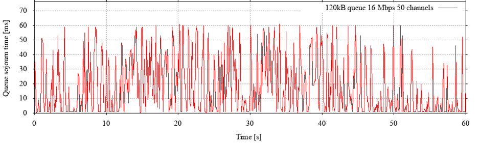 Figure 1: Queue sojourn time on a simulated 16 Mbps geostationary link with up to 50 simultaneous TCP flows from a real-life flow size distribution.
Any truly optimal queue capacity is always load dependent – as in Appenzeller’s study. Note that the queue capacity here is about 1/16th of the BDP – far below the old ‘rule of thumb’. Going by Appenzeller’s theory, we should be having no more than 256 large flows here.
In this experiment, the total number of all flows (long and short) was capped at 50, resulting in an average number of around 37 simultaneously active flows (with the remainder being in the connection establishment phase). An added 40 MB transfer on this link achieves a goodput rate of about 2.3 Mbps.
We can now ask what happens when we vary the load or the queue capacity. If we increase the load, we see more and longer queue overflow events, which affect larger flows. If we cap our load at 60 flows, our 40 MB transfer typically only achieves around 2 Mbps. At 80 flows, this drops to under 1 Mbps. Any gain in link utilization is due to small flows ‘filling’ the queue.
Figure 2 shows that standing queues are starting to develop with no complete queue drainage for seconds at a time. Note, however, that the extra latency added here is only a couple of dozen milliseconds.
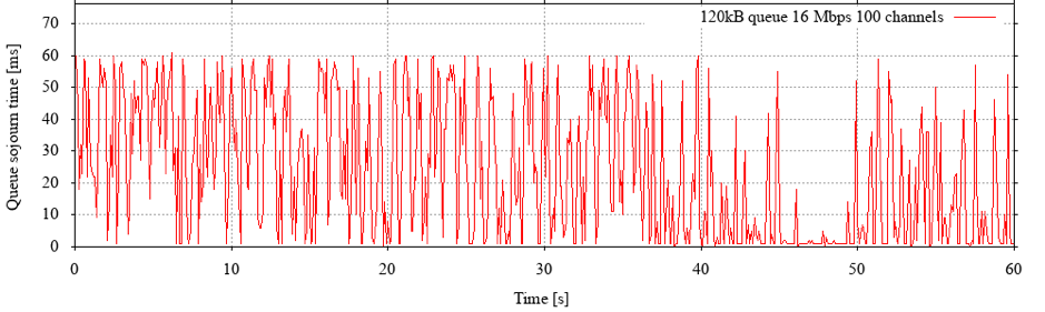 Figure 2: As load increases, standing queues develop – but the queue capacity limits the additional sojourn time.
A larger queue capacity gives large flows, such as our 40 MB flow, a leg up. For example, increasing the capacity to 2000 kB, a much more common value for GEO satellites, sees its average rate climb to over 10 Mbps (>60% of link capacity) when parallel flows are capped at 50.
However, as Figure 3 shows, we now see standing queues almost all the time, which means a longer RTT for everyone – and this slows the short flows down considerably. In short, the rate gain isn’t a gain in efficiency, it’s bought at the expense of the shorter flows.
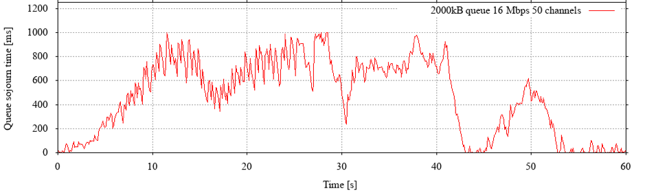 Figure 3: Using commonly deployed queue capacities leads to standing queues that almost never drain once large flows are present. This is only advisable if one truly expects only a very small number of large flows.
Note also the scale on the vertical axis: these standing queues are much longer than the ones we saw before – they can cause the RTT to triple!
If we added more long flows in the 2000 kB scenario, the rates of these flows would collapse rather quickly to values similar to those seen in the 120 kB case. However, the added latency from the standing queues would remain and, in fact, get slightly worse.
Bufferbloat concerns are valid in satellite
Quite how much capacity one should deploy is to an extent a matter of preference. Am I prepared to slow down everyone’s web surfing a little so longer downloads become a bit faster? How important is the performance of real-time applications? It does, however, appear that bufferbloat concerns are valid in the satellite context too.
Contributing author: Lei Qian
Ulrich Speidel is a senior lecturer in Computer Science at the University of Auckland with research interests in fundamental and applied problems in data communications, information theory, signal processing and information measurement. His work was awarded ISIF Asia grants in 2014 and 2016.
The views expressed by the authors of this blog are their own and do not necessarily reflect the views of APNIC. Please note a Code of Conduct applies to this blog.