Striking a balance in fairness

Recently, I’ve been contemplating the concept of fairness, and I see interesting parallels between being a parent and being a network professional. As human beings, we have an inherent, intuitive sense of fairness that manifests itself in various everyday situations. Let me illustrate this idea with a couple of hypothetical scenarios:

Scenario 1: Imagine I’m a parent with four young children, and I’ve ordered a pizza for them to share. If I want to divide the pizza fairly among the children, fairness will mean that each child receives an equal portion — in this case, 1/4 of the pizza.

Scenario 2: Now let’s say I’ve ordered another pizza for the same four children, but one of the kids only cares for pizza a little and will only eat 1/10 of his share. In this situation, it wouldn’t be fair for me to give that child who doesn’t like pizza more than 1/10 of the piece because the excess would go to waste. The fair way to divide the pizza would be to give the child who doesn’t like pizza a 1/10 portion and split the remaining 9/10 evenly among the other three kids.

The approach mentioned in the second scenario represents a principle of fairness known as ‘max-min fairness’, where you allocate resources starting with the least demanding user, then the following least demanding user, and so on.

More broadly, some overarching goals of fairness in the context of networking include:

• Distributing available resources in an equitable manner.
• Isolating badly-behaved users who abuse the system.
• Achieving statistical multiplexing, which means links are divided efficiently.
• Allowing a single-user flow to utilize capacity if no competing flows exist.
• Using a work-conserving scheduler that never leaves a link idle if packets are waiting to be sent.

Max-min fairness

The idea behind max-min fairness is prioritizing smaller demands before allocating excess capacity to larger demands. Specifically, a max-min fair allocation follows these principles:

1. First, fulfil the smallest demand.
2. Once the smallest demand is met, fulfil the subsequent smallest demand.
3. Continue satisfying demands from smallest to largest until all demands are met, or resources are exhausted.
4. If resources remain after all demands are satisfied, allocate the excess to demands fairly.

A common algorithm for achieving max-min fairness operates iteratively:

1. Calculate the fair share for each unsatisfied user.
2. Allocate this fair share to each user.
3. Reclaim any over-allocations and save them as residual capacity.
4. Recalculate fair shares and allocate residual capacity to remaining unsatisfied users.
5. Repeat steps 2-4 until all users are satisfied or resources are fully allocated.

By prioritizing small demands first, max-min fairness aims to maximize fairness for users with varying needs. It ensures resources are divided equitably rather than simply proportionally. The step-wise iterative approach satisfies demands in order from smallest to largest.

Max-min fair bandwidth assignment

Let’s look at an example with a bottleneck link with 10 Gbps of bandwidth shared by four flows. The total demand from the four flows exceeds 10 Gbps. To allocate the 10 Gbps fairly, we’ll go through three iterative rounds; in each round, we allocate the residual bandwidth to the unsatisfied flows (Figures 1, 2, and 3).

Max-min fairness maximizes smaller demands first until resources are exhausted. Flows receive their full demanded bandwidth if possible or the maximum allocation of resources is insufficient, as for Flows 3 and 4. The goal is to prioritize fairness for users with lower demands.

Note that ‘maximizing’ a flow means giving it the highest possible bandwidth allocation according to what remains available. It does not mean fully satisfying each flow’s total demand.

Weighted max-min fairness

Max-min fairness can be extended by assigning weights to demands. Treat a demand of ‘x’ units with weight ‘w’ as separate demands of x/w units each. An allocation is weighted max-min fair if it satisfies max-min fairness for these weighted demands. The algorithm is similar:

1. Calculate the fair share as available resources / total weight.
2. Allocate one fair share unit to each unit of weight.
3. Reclaim any over-allocations.
4. Recalculate and allocate the residual to remaining unsatisfied demands.
5. Repeat until the resources are fully allocated.

This extends max-min fairness by considering demands and weights. It allows a more balanced distribution of resources across varying demands.

Weighted max-min fair bandwidth assignment

In Figures 4 and 5, we iterate in two rounds till no residual bandwidth is left. In step 1, we sum the weights and divide the resource to get the fair share unit per weight and then allocate it to the flows.

Implementation challenges

Unlike the fixed example of kids sharing pizza, network flows are dynamic, constantly changing as flows come and go. This dynamic nature makes it impractical to implement exact max-min fairness.

Instead, a more practical approach is to consider the degree of unfairness, which measures the difference in service received between flows over time. For instance, let’s denote the service received by flow ‘a’ in a time interval [t1,t2] as Sa(t1,t2), and the service received by flow ‘b’ in the same interval as Sb(t1,t2). The degree of unfairness is then given by the difference between these service values, expressed as |Sa(t1,t2)−Sb(t1,t2)|.

A fair method does not favour any specific flow, while an unfair method tends to favour certain flows over others, resulting in some flows receiving more service over time. As time progresses, the time interval [t1,t2] increases, and the difference in the received service also increases, that is, |Sa(t1,t2)−Sb(t1,t2)|.

To determine fairness, we expect that the absolute difference between the received services of flow ‘a’ and flow ‘b’ in any time interval should be less than or equal to some constant, denoted as ‘c’. In other words, |Sa(t1,t2)−Sb(t1,t2)|≤c for every interval.

In the case of weighted fairness, we first normalize the services and then compare the difference in the normalized values, which should also be less than the constant c. The normalized services can be expressed as Sa(t1,t2)/ra and Sb(t1,t2)/rb, where ra and rb are normalization factors for flow ‘a’ and flow ‘b’, respectively.

So, the condition for weighted fairness can be stated as |Sa(t1,t2)/ra−Sb(t1,t2)/rb|≤c. The smaller the difference between the normalized services, the fairer the method is, and if the difference is 0, then the method is perfectly fair.

Buffer management

Background

Before diving into the details, let’s get a high-level understanding of the architecture involved. In most network platforms, buffering is primarily implemented at the ingress side (ignoring smaller egress buffers). The ingress Traffic Manager component is responsible for packet queuing and scheduling. These queues at the ingress side represent the packet queues on the output port, forming what are known as Virtual Output Queues (VOQs). When packets arrive at the ingress, they are enqueued in these VOQs and await a VOQ grant message to proceed to the egress packet processor.

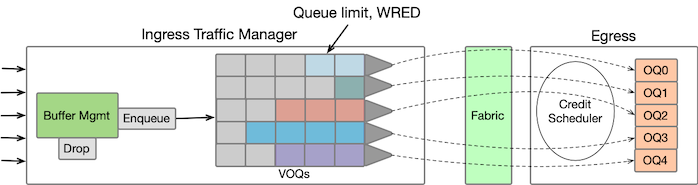
The buffer memory is organized into fixed cell sizes. If a packet is larger than the cell size, it occupies multiple cells plus some overhead for each packet. Regarding buffer allocation, a portion of the buffer memory is reserved for each queue, while the remaining space is shared across all the queues, with allocation occurring on demand. When a packet arrives, the system first checks the reserved pool of the corresponding queue to determine if there is space available. If there is sufficient space, the packet is enqueued in that queue. However, if the reserved pool of the queue is full, the traffic manager looks at the shared pool for buffer space allocation.

A Dynamic Threshold algorithm is employed to make the shared pool buffer space allocation efficient and fair. This algorithm dynamically sets the threshold for each queue based on the buffer utilization. If a queue’s buffer utilization exceeds its dynamic threshold, the incoming packet is dropped to prevent excessive congestion. On the other hand, if the buffer utilization is below the threshold, the shared pool memory is allocated to that queue.

The concept behind the shared pool is to use the buffer memory effectively by leveraging the statistical multiplexing nature of the traffic. This way, the buffer resources are distributed fairly among the active queues, ensuring efficient utilization and congestion control.

Dynamic threshold workings

So, the question that arises now is, how does this dynamic threshold algorithm actually work? In many cases, these details may not be publicly disclosed and may be protected by Non-Disclosure Agreements (NDAs). However, for our purposes, we will primarily refer to the work published in ‘Dynamic Queue Length Thresholds for Shared-Memory Packet Switches‘, which I believe is the most commonly deployed algorithm. Once we understand this then it becomes easier to explore how other implementation approaches tackle similar challenges and enables us to ask the right questions.

Static Threshold and Push Out buffer management schemes

Static Threshold

One approach to buffer allocation involves setting Static Thresholds (STs) per queue and determining the maximum queue length. Cells are accepted if the queue length is below the threshold but dropped if it exceeds the threshold. The challenge with this method is that thresholds remain fixed and don’t adapt to changing traffic loads. If thresholds are too low, queues may discard cells excessively, even with available buffer space. Conversely, if thresholds are too high, some queues may monopolize buffer space, causing starvation for others. Careful tuning and adjustments are required to optimize buffer management based on expected traffic loads, making it less ideal for network operation.

Push Out

With Push Out (PO), an incoming cell can enter a full buffer by displacing another cell. Specifically, the new cell pushes out the cell at the head of the longest queue. The pushed cell loses its buffer space, but the new cell does not take the same position. Instead, it joins its own queue. This lets smaller queues grow by reclaiming space from longer queues.

Key benefits of PO:

• Ensures fairness — shorter queues grow by pushing out longer queues.
• Maximizes efficiency — no starving or idle buffer space.
• Adaptive — queue lengths self-regulate based on activity.
• High overall throughput.

However, PO has some implementation challenges:

• Writing new cells requires extra push-out steps, potentially slowing performance.
• Need to monitor all queue lengths and identify the longest queue.
• Complex for multiple priority traffic classes.
• Overheads to remove and repair pushed-out low-priority cells.

In summary, while PO provides excellent fairness and utilization, its advantages come at the cost of extra complexity. The overheads of push-out operations and length monitoring should be evaluated when considering PO for a specific application.

Dynamic Threshold

In the case of the Dynamic Threshold (DT) scheme, the threshold or maximum queue length is dynamically adjusted based on the unused buffer space. Specifically, the threshold is set to α times the remaining buffer space, where α is a configurable proportionality constant.

T(t)=α∗UnusedBufferSpace=α∗(B−Q(t))

Here, T(t) is the dynamic queue threshold of the port, α is the power of two (positive or negative), B is the total Buffer space, Q(t) is the total buffer occupied at time t, and the sum of all queue lengths.

In a steady state, total buffer occupancy can be given by Q=S∗T+Ω where S is the active queues that are hitting the threshold T and Ω is the space occupied by the uncontrolled queues, which are below the threshold (uncontrolled queues). Substituting this in eq.1 we can find the steady state length Qi of each controlled queue.

T=α∗(B−(S∗T+Ω))

T=α∗B−α∗S∗T−α∗Ω

T+α∗S∗T=α∗B−α∗Ω

T(1+α∗S)=α∗(B−Ω)

T=α∗(B−Ω)/1+α∗S=Qi

When the buffer utilization is low, the thresholds will be higher, allowing longer queues.

Conversely, when the buffer space becomes scarce, the thresholds will be lower to limit queue lengths. This adaptive threshold computation only requires knowledge of the total buffer occupancy and eliminates the need for per-queue monitoring. Implementing α can be easily achieved using a shift register, especially when the values are powers of two, such as 1/16, 1/8, 2, 8, 16, and so on.

Note: An important aspect of the DT approach is that it intentionally maintains a small reserve of buffer space that is not allocated. The remaining non-reserved space is distributed equally among all the active queues. This strategic reserve prevents issues related to starvation and unfairness that might arise with static thresholds.

For example, with α=2, the algorithm aims to maintain each queue’s length at approximately twice the spare buffer capacity. If there is only one active queue, denoted as S=1, then using equation (2), the active queue will be allocated 2/1+2×1×BufferSpace, which amounts to 2/3 of the available buffer space, while the remaining 1/3 is kept reserved and unallocated.

In the case of two active queues, each queue will receive 2/1+2×2×BufferSpace, which equals 2/5 of the free buffer space for each queue. The remaining 1/5 is reserved and remains unallocated.

The key observation is that as the number of active queues increases, the reserved space decreases. This dynamic behaviour ensures that as more queues become active, each queue receives a fair share of the available buffer space, promoting efficient buffer utilization and preventing excessive wastage of resources.

Exploring buffer occupancy and DT through simulations

Let’s delve into the topic through simple discrete event-based simulations. While these simulations may not capture all real-life complexities, they serve to build our intuition. As George Box, the renowned statistician, once said, “All models are wrong, but some are useful.”

Buffer occupancy without DT

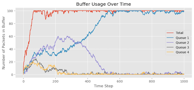
In this scenario, we have a buffer size of 100 cells, and each packet consumes a single cell. Four queues are of equal priority, and packets for each queue are generated using a Poisson distribution, resulting in each queue getting between 0 to 6 packets in each cycle.

In each simulation iteration, packets are added to the buffer if the buffer is not full (occupancy is less than 100). Then, in the same iteration, one packet is removed from each queue in a round-robin (RR) fashion. Since the buffer drain rate is slower than the arrival rate, we can expect the queues to become backlogged. Once the buffer reaches its full capacity, packets start getting dropped.

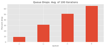
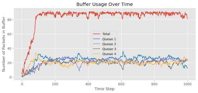
As shown in Figure 7:

Queue	Packets generated	Packets dropped	% Drop
Queue 1	1,255	157	12.51%
Queue 2	1,235	466	37.73%
Queue 3	1,176	649	55.19%
Queue 4	1,277	87	68.36%
Total	4,943	2,145

The simulation plot reveals several key observations:

1. The buffer utilization reaches its maximum capacity, causing packet drops once it hits the limit.
2. Among the queues, Queue 1 has the highest number of packets in the buffer, while Queues 2, 3, and 4 seem to be experiencing starvation with limited access to the buffer.
3. The statistics at the end of the simulation confirm this observation, showing that Queue 3 and Queue 4 experienced the highest number of packet drops.

This outcome is due to the RR approach for adding packets to the buffer. Queue 1 consistently receives priority and consumes the available resources first. As a result, it starves the other queues, leading to fewer packets from Queues 2, 3, and 4 entering the buffer and facing more packet drops.

Because of the randomness involved, we may have observed this just by luck. To ensure our observations’ robustness, we repeated the experiment 100 times and analysed the mean percentage of packet drops for each queue. As depicted in Figure 8, the results consistently show that Queues 2, 3, and 4 are indeed experiencing starvation, leading to a higher percentage of packet drops than Queue 1.

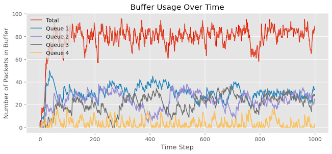
Buffer occupancy with DT

Let’s replicate the experiment with a DT. We will add this condition to our code which checks if the current queue length is less than the α×(buffersize−buffer_occupied)) with α=2.

if self.queue_packets[packet.source] <
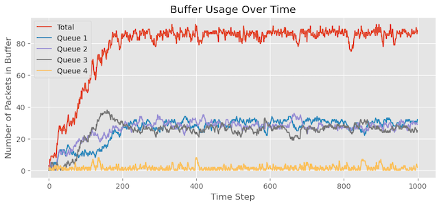
        packet.alpha * (self.limit - len(self.packets)):

Figure 9 showcases the results of our simulation, and we can derive several observations from it:

1. In contrast to the previous experiment, the buffer utilization does not reach its maximum capacity. This behaviour is associated with the DT mechanism, which deliberately reserves some buffer space.
2. We previously discussed the steady-state queue allocation formula: α/1+α×S×BufferSpace. With four active queues, each queue is allocated approximately 2⁄9 of the buffer space (around 22 cells), while 1⁄9, that is, 11 cells from the 100 cells available are reserved. Thus, the maximum expected utilization is approximately 89 cells.
3. It is evident that Queues 2, 3, and 4 are not experiencing starvation as they did in the previous experiment. Most queues maintain a state of equilibrium with resource allocation.

As shown in Figure 9:

Queue	Packets generated	Packets dropped	% Drop
Queue 1	1,250	243	19.44%
Queue 2	1,150	128	11.13%
Queue 3	1,183	161	13.61%
Queue 4	1,248	227	18.19%
Total	4,831	759

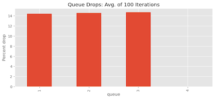
Once again, to ensure the reliability of our findings, we repeat the experiment 100 times and observe the mean percentage of packet drops for each queue. As shown in Figure 10, it’s evident that the queue allocation is now much fairer, no queue is experiencing starvation, and the buffer drops for each queue are similar.

Buffer occupancy with DT and Weighted RR

In this scenario, we introduce a priority scheme to prioritize Queue 4 over the other queues. Initially, each queue had a priority of 1 buffer occupancy, but now we will increase the priority of Queue 4 to 2. This change means that twice the number of packets will be drained from the buffer for Queue 4 in each cycle compared to other queues. As a result, the buffer occupancy for Queue 4 packets will be lower than the other queues.

It’s important to clarify that high weights in this context do not determine the priority to access the buffer initially. Instead, the weights define the order in which packets are drained from the buffer for the already present packets.

Figure 11 illustrates the output of a single run, aligning with our expectations. Queue 4 exhibits minimal buffer occupancy, and the number of packet drops for Queue 4 is zero. Additionally, the remaining queues, all equal priority, share similar buffer occupancy.

As shown in Figure 11:

Queue	Packets dropped
Queue 1	128
Queue 2	164
Queue 3	167
Queue 4	0
Total	459

By repeating the experiment 100 times and analysing the mean results, we observe that Queue 4 experiences no packet drops.

Changing the traffic assumptions

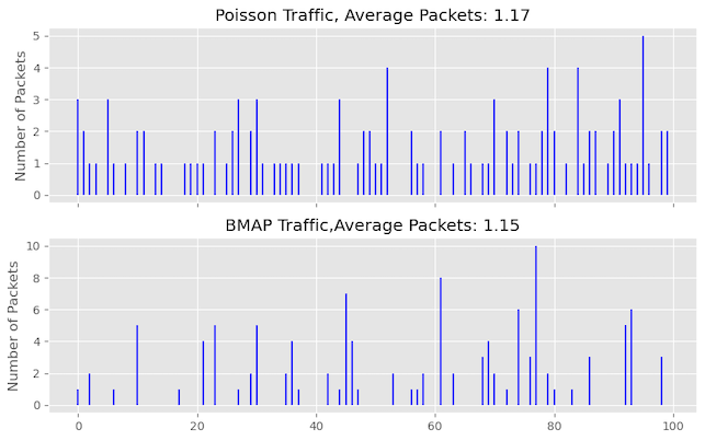
Now, we will investigate the impact of traffic with a more bursty nature. To achieve this, we will modify the previous assumption of Poisson traffic and instead use the Batch Markovian Arrival Process (BMAP) to generate packets. BMAP generates packets that exhibit more bursty behaviour than packet arrivals in Poisson traffic.

Figure 13 shows the difference in the number of packets arriving for each time unit between Poisson traffic and BMAP traffic scenarios. In the case of Poisson traffic, the packet arrivals are more consistent and evenly spread over time. Conversely, with BMAP traffic, packet arrivals are less frequent. Still, when they occur, they are more bursty, resulting in periods of low packet arrivals followed by sudden bursts of multiple packets arriving quickly.

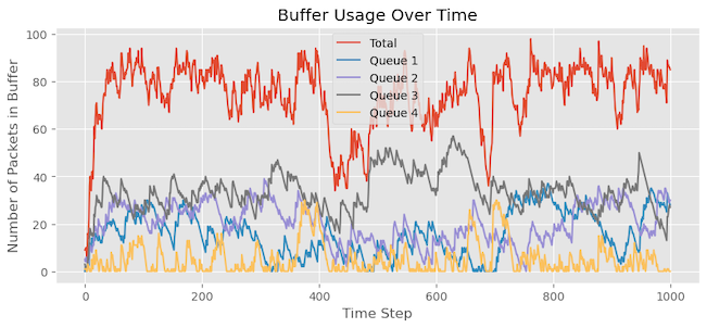
Buffer occupancy with DT and WRR for bursty traffic

In this scenario, I have made the traffic more bursty in nature while maintaining Queue 4’s higher weight (weight = 2) compared to other queues. Comparing the graph with the previous experiment, we can observe that more packets for Queue 4 are staying in the buffer. We also notice that Queue 4 experiences now some packet drops that we didn’t see earlier.

As shown in Figure 14:

Queue	Packets dropped
Queue 1	257
Queue 2	145
Queue 3	211
Queue 4	18
Total	631

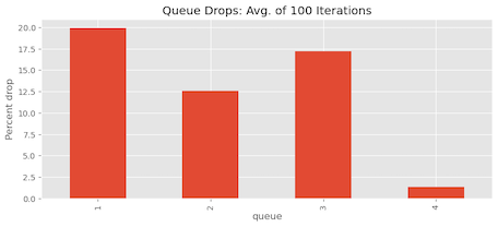
Repeating the experiment multiple times and analysing the mean results, we find that on average, there are 1.37% packet drops for Queue 4:

Queue	% Packets dropped
Queue 1	19.95%
Queue 2	12.54%
Queue 3	17.18%
Queue 4	1.37%
Total	631

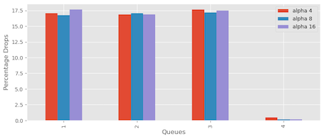
One approach we can take to address the packet loss issue for Queue 4 is increasing the alpha value from 2 to 4. By doing so, Queue 4 will be allocated a larger portion of the buffer than the other queues. The aim is to determine if this adjustment reduces or eliminates the packet drops for Queue 4. However, upon analysing the statistics, we observe that although the packet drops have decreased, they have not been completely eliminated:

Queue	Packets dropped
Queue 1	57
Queue 2	134
Queue 3	432
Queue 4	14
Total	637

Figure 17 shows the impact of different alpha values of 4, 8, and 16. The purpose was to observe how adjusting the alpha value influences packet drops in the system. The findings revealed that increasing the alpha value from 4 to 8 and 16 did improve packet drop reduction but did not remove them altogether.

Let’s summarize our progress so far:

• We have explored the DT scheme for buffer management, understanding how it dynamically adjusts buffer sharing based on the unused buffer capacity. The threshold value changes adaptively according to the available buffer space.
• As confirmed by our simulations, the DT scheme strategically reserves a small buffer space and distributes the remaining buffer equally among the active queues.
• Through comparisons between scenarios with and without the DT, we have observed how it enhances fairness in buffer allocation among active queues and effectively prevents starvation.
• We have also studied buffer draining using WRR and its impact on buffer occupancy.
• To assess the scheme’s performance under bursty traffic conditions, we introduced more bursty traffic using BMAP. We observed that increasing the alpha value improved the loss percentage but we were not able to get rid of the packet loss completely.

It’s important to highlight that we wholly ignored the two key factors here, the packet size distribution and the congestion control backoff behaviour when they observe packet loss. This was because the amount of code I had to write was much more effort than the time I had.

RR and DRR: Ensuring fairness in buffer draining

In the context of buffer draining, we have employed both RR and WRR scheduling techniques. While the basic RR approach can achieve fairness when all queues have equal weights and uniform packet sizes, it will lead to imbalances when the queues contain packets of varying lengths. For instance, if one queue primarily holds 500-byte packets while another mainly contains 1,500-byte packets, the RR approach may result in unequal shares for the queues, despite having equal priority.

To address this challenge, the Deficit Round-Robin (DRR) scheduling algorithm, proposed by Sheerhar and Varghese in ‘Efficient Fair Queuing Using Deficit Round-Robin‘, comes to the rescue.

DRR ensures fairness even when the packets have different sizes. It achieves this by introducing a ‘deficit counter’ representing the number of bytes a queue can transmit when its turns come. Additionally, it maintains a ‘quantum’ counter, which specifies the number of bytes added to the deficit counter of a queue at each round. You can think of the quantum as a credit accumulating with each iteration.

The operation of a DRR scheduler can be summarized as follows:

1. Packets from queues are transmitted in a RR fashion, with the deficit counter initialized to zero.
2. Before servicing a flow, the quantum value is added to the deficit counter of that flow: deficit counter += quantum.
3. A packet from a queue is only transmitted if the deficit counter is greater than or equal to the length of the packet: deficit counter >= packet length.
4. If a packet is transmitted, the deficit counter of that flow is updated by subtracting the number of bytes in the transmitted packet: deficit counter -= #bytes in the packet.

By incorporating the DRR algorithm, we can ensure fairness in buffer draining, even when the packets have varying sizes across different queues. This approach promotes more efficient and equitable utilization of network resources.

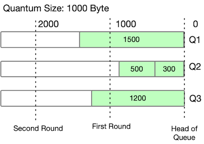
As an example, consider two iterations with a quantum size of 1,000 bytes:

Count	Quantum size	Packets served
First iteration
A count	1,000	No packet is served since 1,500 > 1,000 deficit counter
B count	200	Both packets are served
C count	1,000	No packet is served since 1,200 > 1,000 deficit counter
Second iteration
A count	500	Packet is served: 2,000 – 1,500 = 500
B count	0	0
C count	800	Packet is served: 2,000 – 1,200 = 800

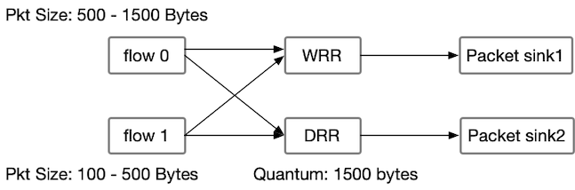
We can also compare the schemes using discrete event simulation. We consider two flows: Flow 0 and Flow 1. Flow 0 generates packets ranging from 500 to 1,500 bytes, while Flow 1 generates packets ranging from 100 to 500 bytes. Both flows are directed to two different scheduling algorithms: WRR and DRR schedulers.

For the DRR scheduler, we have set the quantum size to 1,500 bytes. The simulation captures the arrival of packets from both flows at the packet sink side under these scheduling schemes. By analysing the simulation results, we can observe how the packets from each flow are processed and drained using WRR and DRR schedulers, respectively.

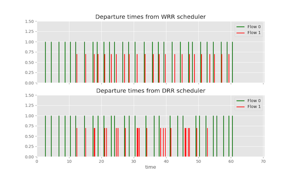
The results of the simulation indicate that the WRR scheduler simply alternates between Flow 0 and Flow 1 in a RR fashion. However, the DRR scheduler sends more packets from Flow 1 in each iteration, demonstrating the fair and efficient buffer draining achieved by the DRR algorithm.

Conclusion

In this post, we explored fairness in buffer allocation and packet scheduling techniques. We identified the limitations of fixed thresholds and introduced DTs to adapt buffer sharing based on available capacity, promoting fairness and preventing starvation.

The DRR scheduling algorithm addressed fairness concerns with varying packet sizes, ensuring equitable buffer utilization. Bursty traffic simulations showed the importance of alpha values in improving fairness and reducing packet drops, though complete elimination of drops was not achieved.

While our exploration did not consider packet size distribution and congestion control, it highlighted the significance of fair buffer allocation and efficient scheduling for network performance.

I hope you find this helpful, and if you have any ideas or suggestions, please don’t hesitate to contact me.

Diptanshu Singh is a Network Engineer with extensive experience designing, implementing and operating large and complex customer networks.

This post (and further reading) was originally published on Diptanshu’s blog.

Rate this article

---

The views expressed by the authors of this blog are their own and do not necessarily reflect the views of APNIC. Please note a Code of Conduct applies to this blog.