

The Internet has recently undergone an unprecedented set of changes with the exhaustion of IPv4 addresses, one of which has been the adoption of IPv6.
There are many researchers and engineers tracking this adoption and figuring out how people use IPv6 to assign addresses to systems, how many systems with IPv6 addresses exist, and how people try to avoid using IPv6.
This research is particularly difficult as the simple brute-force technique of checking all available addresses – that works well with IPv4 – is not feasible for IPv6 for the fact that there are simply too many addresses.
That said, several techniques have been developed – a collection of which can be found in RFC7707 – and one of which, proposed by Peter van Dijk, that we have adapted and described here.
Reverse DNS
Reverse DNS is a special DNS top-level zone (in-addr.arpa. for IPv4 and ip6.arpa. for IPv6), which can be used to obtain fully qualified domain names for an IP address. For example, the address 2001:DB8::1 has the reverse record 1.0.0.0.0.0.0.0.0.0.0.0.0.0.0.0.0.0.0.0.0.0.0.0.8.b.d.0.1.0.0.2.ip6.arpa..
Such a zone can be enumerated for IPv6 to obtain possibly allocated addresses. To do this, you use a special semantic of a DNS response code. If RFC1034 is implemented correctly, as clarified in RFC8020, then rcode 3 in the DNS, also known as NXDOMAIN, has a special meaning:
”’NXDOMAIN means that the authoritative server has no data at the requested node of the DNS tree, and knows that there is no data anywhere thereunder.”’
The idea behind this semantic is easier negative caching, which addresses various DNS-based attacks. However, it also allows us to identify possible allocated IPv6 addresses.
Enumerating zones
To enumerate a zone using this semantic, you must start with a prefix. Let’s use our example from before, considering the /64 2001:DB8::1 is in: 0.0.0.0.0.0.0.0.8.b.d.0.1.0.0.2.ip6.arpa..
When requesting 0.0.0.0.0.0.0.0.0.8.b.d.0.1.0.0.2.ip6.arpa. (note the extra zero), the authoritative server replies with rcode 0, NOERROR. This is because there is something under that node in the tree, namely the reverse record for our example address.
However, if we request 1.0.0.0.0.0.0.0.0.8.b.d.0.1.0.0.2.ip6.arpa., we receive an rcode 3, NXDOMAIN response. Subsequently, we can do this for all levels of the DNS tree, only descending into branches that returned NOERROR.
Going global
This technique works on single prefixes, however, it does not easily work on the whole reverse zone for all addresses. To run van Dijk’s technique on an Internet scale, there were three key issues that we had to address.
1. Seeding
On the Internet, many things can go wrong – we may encounter DNS servers that always send NXDOMAIN, which means we miss out on zones.
To overcome this and get an ideal zone-width, we seed our dataset with a list of currently announced IPv6 prefixes.
2. Parallelizing
We must parallelize, if we want to enumerate a lot of zones in a structured manner. To do this, we conduct an iterative depth-first search.
We start at our seed-sets and only enumerate all zones up to a certain depth. If the seed is deeper in the tree than we want to go, we crop the seed, and add both the cropped and the seed value to our output set.
With this approach, we can paralellize over all these inputs. The results are then used as the input for the next step.
3. Dynamic Zones
Some operators, mostly ISPs, will dynamically generate reverse zones for IPv6 networks up to a /32. In such cases, every possible address of a prefix seemingly has a reverse record.
Even for a small /64, this leads to a lot of dynamically generated data that takes weeks to retrieve but holds no information on whether addresses are allocated.
We opted to identify such zones by querying 16 possible full-length records (32 levels deep) before enumerating a prefix further. If these all seemed to exist, we considered the zone dynamically generated, and skipped it.
What we can see
By integrating our improvements, we can apply van Dijk’s technique to get a more global picture.
From our data we can observe how operators allocate IPv6 addresses. For example, we can look at datacentres of major SaaS providers, while they roll out new systems.
In our initial scans, we were able to find 5.8 million unique IPv6 addresses. Subsequent scans with a better load balancing found more than 10 million unique possibly allocated IPv6 addresses.
As you can see in Figure 1 and 2, the operators allocate addresses and networks in three different regions sequentially.
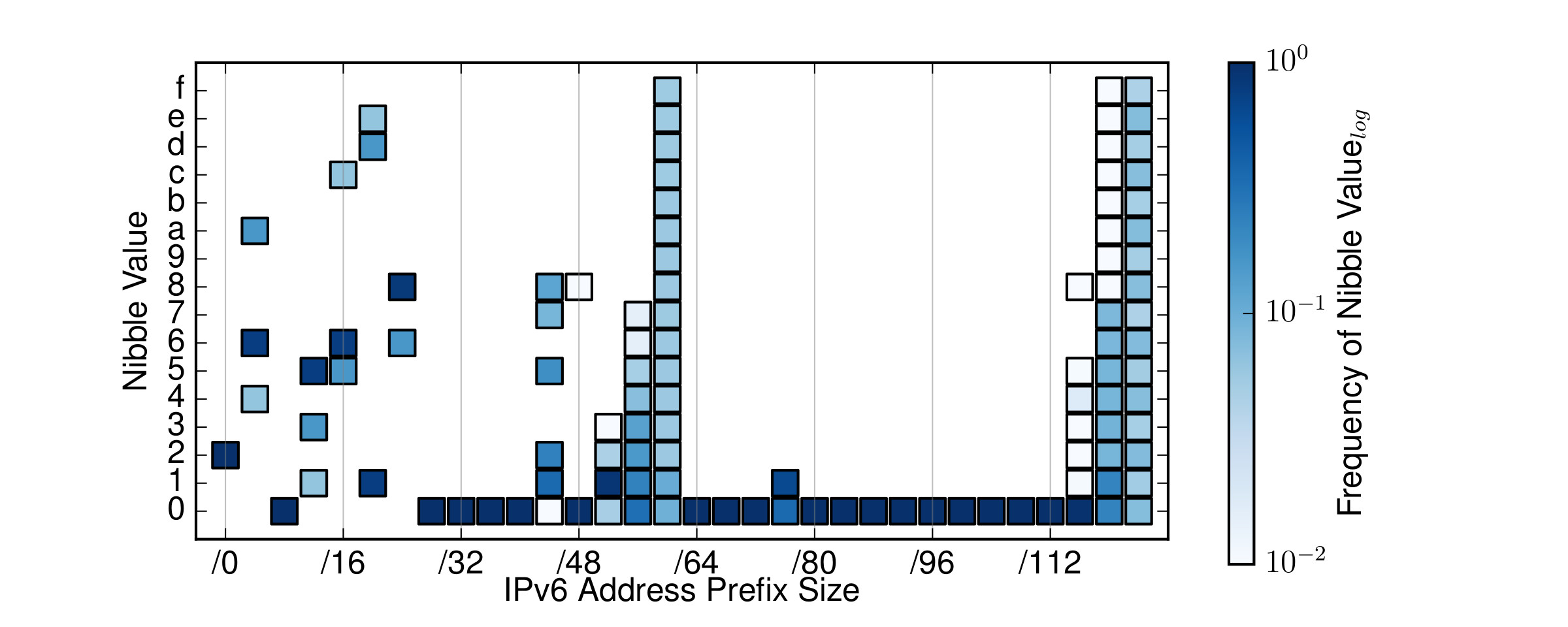
Figure 1: IPv6 address prefix size allocations for SaaS providers.
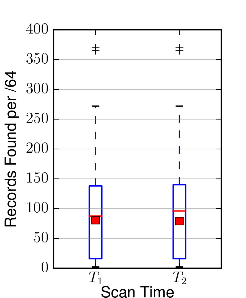
Figure 2: Box plot showing records found per /64 for SaaS providers.
At the same time, on average, they keep the number of systems per /64 under 256.
This indicates that they allocate a /64 per physical segment and are restricted by the size limitations of a /24, which is possibly their standard IPv4 allocation in a dual-stack scenario.
If you want to learn more about this technique and our findings watch a recent presentation we gave (below) and read our whitepaper.
Tobias Fiebig is a researcher at TU Berlin, with a focus on network measurement and network security. You can learn more about his work at http://aperture-labs.org.
The views expressed by the authors of this blog are their own and do not necessarily reflect the views of APNIC. Please note a Code of Conduct applies to this blog.