Rate-based versus credit-based flow control: Part 2 — Notes on flow control

In this series ‘Notes on flow control’ Diptanshu Singh shares notes from his studies of scheduling mechanisms used in router architectures. The series began with principles of flow control and is now covering two widely used flow control mechanisms: Rate-based and credit-based.

In this post, I will compare rate-based and credit-based flow control mechanisms, and the distinct characteristics and tradeoffs that influence system design and performance.

Rate-based flow control

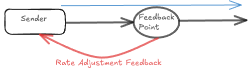
In rate-based flow control, a contention point (switch, network interface controller, and so on) measures some local metric that correlates with congestion (queue depth, output link use, latency, and so on) and feeds back a target sending rate or rate adjustment to the upstream sender. The sender then shapes its traffic so that its instantaneous departure rate follows that target.

Feedback style can be either absolute or differential.

In the case of absolute, the old rate is replaced by the new rate:

$$\mathrm{\lambda <!--\; \lambda \; -->}\to <!--\; \to \; -->{\mathrm{\lambda <!--\; \lambda \; -->}}_{new}$$

In the case of differential, rate adjustment takes the form of ‘speed-up by △’ or ‘slow-down by △’, where △ is expressed as a percentage.

Absolute control mechanisms that attempt to fully correct transmission rates within a single RTT tend to be coarse and may overreact. In contrast, differential control makes smaller adjustments, requires less signalling overhead, and is better suited to tracking traffic patterns that change over time.

Simplistic rate-based flow control (XON/XOFF)

The simplest form of differential rate-based flow control is a two-level threshold-based scheme, commonly called XON/XOFF (or ON/OFF) flow control. Its operation is straightforward:

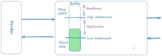
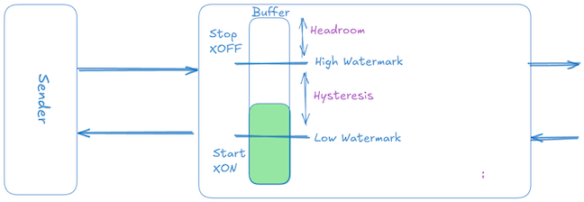
• When the receiver’s buffer occupancy hits a high watermark threshold, it sends an XOFF signal, instructing the sender to immediately stop transmission (sender rate → 0).
• Once the receiver buffer drains and occupancy falls below a low watermark threshold, it sends an XON signal, instructing the sender to resume transmission at the full, unrestricted rate (sender rate → peak).

Although this method is trivial to implement and widely used in standards like Ethernet Pause (802.3x) and Priority Flow Control (802.1Qbb), it is inefficient in terms of buffer usage. The inefficiency arises primarily because XON/XOFF control signals are threshold-triggered rather than continuously updated based on precise buffer state, unlike credit-based flow control.

Propagation delay overshoot

When the receiver’s buffer occupancy reaches the high watermark threshold, it sends an XOFF signal back to the sender. However, due to the propagation delay, the sender will continue to transmit packets until it actually receives and processes the XOFF signal. This delay leads to an overshoot in buffer occupancy, requiring sufficient extra space in the receiver buffer to accommodate packets already ‘in-flight’.

To estimate the size of the overshoot caused by in-flight packets, we can take a sum of reaction data, wire data and small far-end data. ‘Near-end’ and ‘far-end’ are relative to the receiver.

Reaction data: From the instant the packets in the near-end buffer cross the XOFF threshold until the far-end stops transmitting. This is basically the time it takes to generate XOFF, transmit it back to the sender, and the action time for the sender to pause out-bound transmission.

$$\text{Reaction data}=R\times <!--\; \times \; -->(T_{gen}+\text{Link delay(one way)}+T_{action})$$

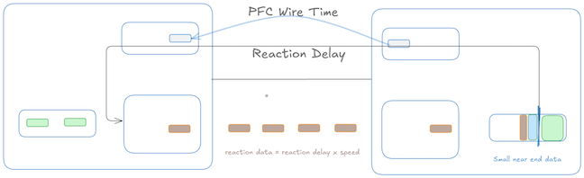
Wire data: The time after the last bit has left the far-end but has not yet reached the near end.

$$\text{Wire data}=R\times <!--\; \times \; -->\text{Link delay(one way)}$$

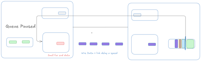
There is some minor residual data from small far-end and near-end data which is in-flight in addition to the reaction and wire data. So the additional buffer space (also known as ‘headroom buffer’) needed to accomodate data from the propagation delay overshoot is:

$$\text{Headroom}=\text{Reaction data}+\text{Wire data}+\text{Small near-end data}+\text{Small far-end data}$$

I have simplified the factors affecting the calculation of the required headroom buffer. It is worth noting that, in addition to what I have mentioned, link delay is also a factor. As the link length starts growing, link delay becomes the dominating factor.

Hysteresis margin to avoid oscillation

If the reciever sends the XON signal as soon as the data in the buffer falls below the XOFF threshold, the sender starts transmitting again while the reciever local-queue still holds the residual bytes generated during the previous pause window. This can cause the buffer to immediately reach the XOFF threshold again, creating oscillations between XON and XOFF states known as chattering.

To avoid rapid oscillation between XON and XOFF states, the receiver does not immediately send the XON signal upon dropping slightly below the XOFF threshold. Instead, a significant gap — the hysteresis window — is deliberately maintained between the high (XOFF) and low (XON) thresholds. Typically, this hysteresis window is a full reaction data worth of packets (or some percentage of the XOFF threshold). This maintains system stability by ensuring that by the time transmission restarts the buffer occupancy is comfortably below the high threshold.

Impact of link delay and rate

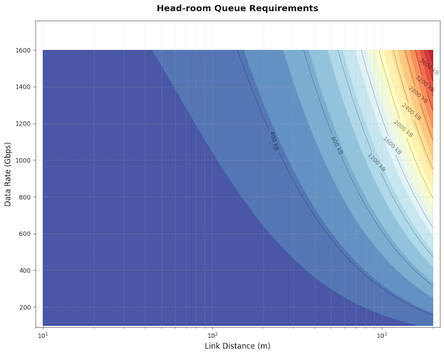
Earlier we discussed how the required headroom buffer space can be calculated, with reaction data and wire data as the main contributing factors. As either distance or data rate increases, more bytes are ‘in-flight’, requiring larger buffers to avoid packet loss.

The plot below shows that at shorter distances, buffer requirements are modest and dominated primarily by fixed silicon delays (interface and higher-layer delays), but as the link length or speed grows beyond a certain point, the buffer requirement dramatically increases, driven predominantly by the propagation delay (which adds additional bytes proportional to the bandwidth-delay product (BDP).

The plot assumes maximum transmission unit (MTU) is 9,216 bytes, XOFF frame size is 64 bytes, interface delay is 250ns, and higher-layer delay is 100ns.

Credit-based flow control

In credit-based flow control, communication occurs between a sender and receiver about buffer availability at the receiver, with a one-RTT delay.

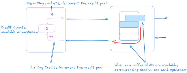
The sender uses ‘credits’ to regulate transmission, with each credit representing space in the receiver’s buffer. Transmission is permitted only when the sender has available credits. Upon processing a packet, the receiver returns a credit to the sender, signalling that buffer space has become available again.

RTT defines the control-loop delay, during this window sender’s view of the buffer is stale. The receiver needs to have enough space in the buffer to hold the data transmitted by the sender in one RTT.

How big should the receiver’s buffer be to ensure that the communication remains loss-free and the receiver always has enough data to keep its outgoing link fully used despite the presence of an RTT delay?

A buffer of one BDP is needed to keep the link loss-free while maintaining full use. At the sender, the data only leaves if a credit (representing a free slot) has already arrived. Overflow is impossible even under abrupt stop/start conditions because:

$$buffer\ge <!--\; \ge \; -->Rate\times <!--\; \times \; -->RTT$$

Let’s look at a toy example, by assuming:

• Link Rate = 1 cell / time unit (tu).
• One-way delay = 3 time units.
• RTT = 6 time units.
• BDP = Rate x RTT = 1 x 6 = 6 cells.
• Receiver Buffer = 6 cells.

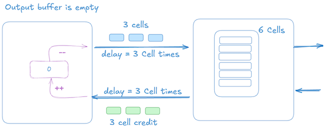
In the initial state (t=0):

• The receiver has dequeued 3 cells, which has resulted in sending 3 more credits back to the sender. The receiver buffer is empty at this point, but the receiver has just become congested, resulting in no dequeue happening.
• The sender already has 3 credits from earlier dequeues.

The picture below shows that 3 cell credits are in transit, the sender has sent 3 data cells towards the receiver, and its credit count is 0.

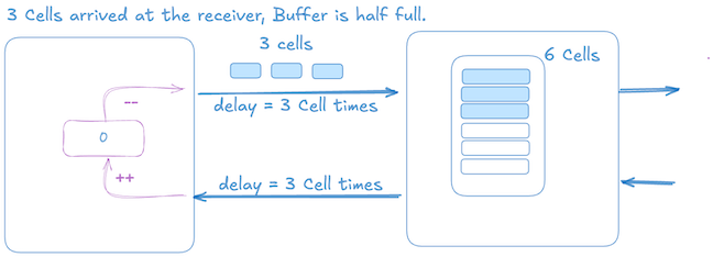
Once the 3 cells arrive at the receiver, the sender also gets 3 more credits that results in transmitting 3 more data cells, which the receiver can accommodate. At this point, the sender is stalled until it gets more credits.

Below is a time sequence diagram (click to enlarge) which goes through all the events in more detail.

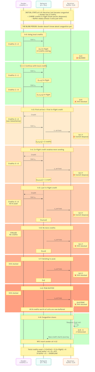
At time 6, the buffer reaches 4/6 occupancy. The sender has consumed all 6 credits and sent 6 cells. This demonstrates why we need at least 6 cells of buffer, otherwise, cells arriving after time 6 would be dropped. A reader can play the same scenario with the initial conditions and with a buffer of less than 6, and observe that it will result in a drop at the receiver.

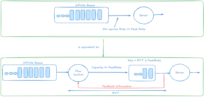
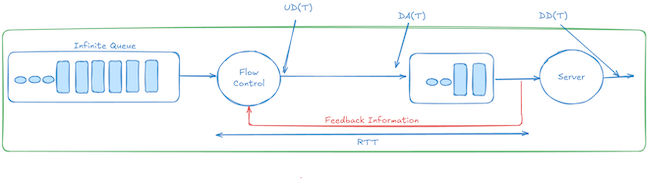
Infinite‑queue equivalence

Infinite-queue equivalence is a conceptual model that says a finite, credit-protected buffer at the receiver sized to the BDP behaves as if there were an infinite queue immediately downstream of the sender, before the link.

$$\text{BDP}=R\times <!--\; \times \; -->RTT$$

Losses are prevented because the sender’s transmission rate is controlled by the arrival of credits from the receiver. When the real downstream buffer fills, credits stop arriving, and the sender slows down — creating the illusion of an infinite queue that never overflows.

To understand how the infinite-queue equivalence theorem works, let’s assume that we have:

• DD(t): Cumulative downstream departures physically exiting the downstream node up to time t.
• UD(t): Cumulative upstream (sender) departures up to time t. It’s the data sent by the upstream node, and it depends directly on credits returned after downstream departures.
• DA(t): Cumulative data arrivals into the downstream buffer.
• Service‑rate constraint: The amount of data exiting the node is less than or equal to Rate × d, where d is the time delta between t + d and t:

$$0\le <!--\; \le \; -->DD(t+d)-<!--\; -\; -->DD(t)\le <!--\; \le \; -->Rd$$

Credit rule: At any instant, the sender owns exactly the credits that represent free slots in the receiver buffer. Immediately after start‑up, the sender holds one BDP-worth of credits.

Upstream departures: The sender can transmit only when it owns credits, and each departure consumes one credit.

$$UD(t)=DD(t-<!--\; -\; -->RTT)+RTT\times <!--\; \times \; -->R$$

At the start, the sender has exactly one BPD-worth of credits. This is the initial credit window. After initial credits are spent, new credits arrive exactly one RTT after downstream data is transmitted. Thus, the total sent upstream at time ‘t‘ is the total transmitted downstream by (t - RTT) plus initial credits.

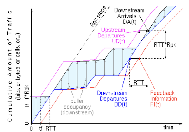
Downstream arrivals: Since data takes exactly one RTT to travel from upstream to downstream, the Downstream Arrival function DA(t) can be given as:

$$DA(t)=UD(t-<!--\; -\; -->RTT)=DD(t-<!--\; -\; -->RTT)+R\times <!--\; \times \; -->RTT.$$

This means that the data entering the downstream buffer at time ‘t’ corresponds exactly to the downstream departures one RTT earlier, plus the fixed initial credit window.

Buffer occupancy: The occupied buffer can be represented as the difference between data packets arriving and data packets departing.

$$BO(t)=DA(t)-<!--\; -\; -->DD(t)=R\times <!--\; \times \; -->RTT-<!--\; -\; -->[DD(t)-<!--\; -\; -->DD(t-<!--\; -\; -->RTT)].$$

The bracketed term [DD(t) − DD(t − RTT)] is non‑negative and at most R × RTT by the service‑rate constraint, so:

$$0\le <!--\; \le \; -->BO(t)\le <!--\; \le \; -->R\times <!--\; \times \; -->RTT=\text{BDP}.$$

Hence, the buffer never overruns, and from the sender’s viewpoint, the system behaves as if any excess data were ‘pushed back’ into an infinite queue.

BDP sufficiency and necessity (corollary)

The proof establishes that a buffer of exactly one BDP is sufficient for lossless operation.

Conversely, if the buffer were any smaller, the worst‑case blind‑period injection of R × RTT bytes could overflow it, so the BDP size is also tight. This formalizes the sizing rule introduced in the credit‑based flow control section of this blog post, and demonstrated with an example.

Comparing credit-based vs rate-based (XON/XOFF)

We looked at both credit-based and rate-based (or XON/XOFF) flow control mechanisms. As the link distance, link rate, or both increase, credit-based schemes require less buffer than rate-based schemes.

Credit-Based: The minimum buffer requirement is precisely one BDP, ensuring overflow is inherently prevented:

$$B_{min}=R\times <!--\; \times \; -->RTT(\text{one BDP})$$

XON/XOFF: The buffer headroom for XON/XOFF includes three distinct components:

• Reaction Data: Bytes transmitted during pause frame generation, propagation, and sender pipeline drain.

$$R(T_{gen}+T_{link}+T_{act})$$

• Wire Data: Bytes already in transit on the link.

$$R{T}_{link}$$

• Hysteresis: Typically, another full reaction-data segment to prevent frequent toggling (XON/XOFF chatter).

The total buffer headroom requirement thus becomes:

$$\text{Headroom}=R(T_{gen}+T_{link}+T_{act})+R{T}_{link}+\text{Hystersis (Another reaction data worth of space)}$$

Because both reaction and wire-data terms scale linearly with link length, the overall buffer demand for XON/XOFF increases faster than BDP does over longer distances.

In the next post…

While both rate-based and credit-based approaches to flow control regulate traffic and prevent congestion, their implementation and behaviour differ significantly. Next, we’ll look at how flow control is handled in switch Application-Specific Integrated Circuits (ASICs), where hardware constraints and architectural choices play a critical role.

Diptanshu Singh is a Network Engineer with extensive experience designing, implementing and operating large and complex customer networks.

This post was adapted from the original on his blog.

Rate this article

---

The views expressed by the authors of this blog are their own and do not necessarily reflect the views of APNIC. Please note a Code of Conduct applies to this blog.