

In this series ‘Notes on flow control’, Diptanshu Singh shares notes from his studies of scheduling mechanisms used in router architectures. The series begins by looking at the principles of flow control, and will cover mechanisms and implementations in future articles.
Flow control is a fundamental concept in the design of high-performance networks. While reviewing the scheduling mechanisms used in router architectures, I took the opportunity to revisit the core principles of flow control, examine its various mechanisms, and reflect on their practical implications. My notes outline key models, compare typical schemes, and highlight relevant system-level considerations.
I’ve adapted those notes into a three-part series:
- Post 1: Principles of flow control (this post).
- Post 2: Rate-based versus credit-based flow control.
- Post 3: Flow control in Application-Specific Integrated Circuits (ASICs).
In this, the first post of the series, we’ll explore some of the core concepts of flow control.
Principles of flow control
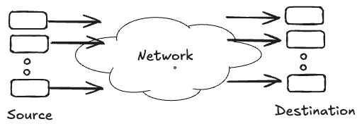
Flow control is a fundamental problem in feedback control for network communications. At its core, flow control addresses two critical questions that every network must solve:
- How do sources determine the appropriate transmission rate?
- How do sources detect when their collective demands exceed the available network or destination capacity?
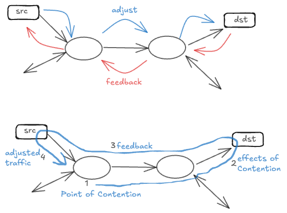
The solution lies in establishing effective feedback mechanisms from network contention points and destinations back to the sources, creating a self-regulating system that maintains network stability and performance.
The fundamental role of round-trip time
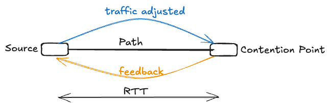
Round-trip time (RTT) serves as the fundamental time constant in any feedback-based flow control system. RTT represents the minimum delay that a source must wait before observing the effects of its transmission decisions. When a source begins transmitting, it will only learn about the impact of that transmission in one RTT after it has started — the time it takes for a packet to travel to the destination and back.
Similarly, when congestion occurs at a contention point in the network, the corrective effects of any feedback mechanism will only manifest at that contention point one RTT after the congestion event has occurred. This inherent delay creates what we call a ‘blind mode‘ transmission — a period during which sources must transmit without knowledge of current network conditions.
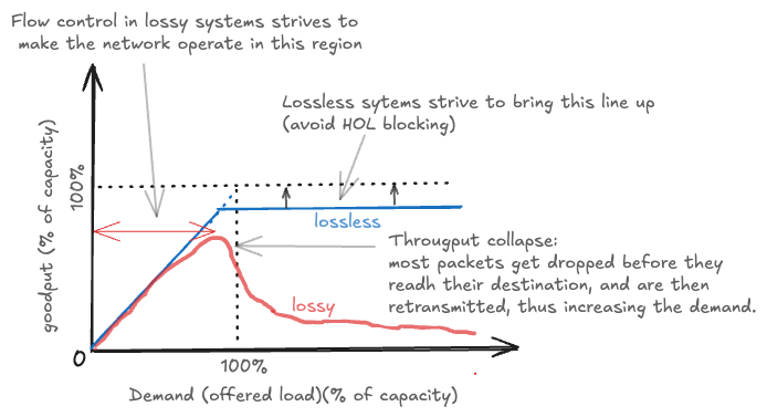
Lossy vs lossless flow control paradigms
Flow control systems fundamentally divide into two paradigms, each with distinct characteristics inherited from different engineering disciplines.
Lossy flow control, inherited from communication engineering traditions, accepts that buffer overflows may occur and packets can be dropped. While this approach appears simple, it introduces significant complexity. Lost data necessitates retransmissions, which waste valuable communication capacity and create a gap between goodput (useful data delivered) and throughput (total data transmitted). Maintaining satisfactory goodput under lossy conditions requires carefully designed protocols that can efficiently detect losses and orchestrate retransmissions without exacerbating congestion.
In contrast, lossless flow control guarantees that buffers will never overflow, ensuring no data loss occurs. This approach, inherited from hardware engineering where processors never drop data, eliminates wasted communication capacity and minimizes delay. However, lossless systems introduce their own complexities, requiring multi-lane protocols to avoid head-of-line (HOL) blocking and to break potential cyclic buffer dependencies that can create deadlock. The choice between lossy and lossless approaches profoundly impacts system architecture and performance characteristics.
Classification of flow control schemes
Flow control schemes can be classified along multiple dimensions, each representing different design choices and tradeoffs. The first major distinction is open-loop, closed-loop and hybrid control. Open-loop admission control makes static decisions at connection setup time, while closed-loop adaptive flow control continuously adjusts during runtime based on current conditions.
Flow control mechanisms can be further characterized by whether they use implicit or explicit feedback, whether control is applied end-to-end or hop-by-hop, whether traffic is regulated indiscriminately or per-flow, and whether transmission is governed by rate-based or credit-based techniques. Credit-based systems are typically closed-loop and hop-by-hop, while rate-based systems can be either open- or closed-loop, and implemented as either end-to-end or hop-by-hop control.
Open vs closed-loop flow control
Open-loop control
Open-loop flow control requires a source to request and secure network resources before initiating data transmission. After making this request, the source must await approval, incurring at least one RTT of additional delay compared to closed-loop methods. Once approved, the source transmits at the allocated, reserved rate.
While this approach guarantees predictable service quality, it comes with significant drawbacks. Reserved but idle resources cannot be dynamically reallocated to other sources, potentially leading to poor resource utilization. Historically, open-loop control has its roots in telephony systems, inheriting a binary approach to resource allocation — either admit new flows at the risk of degraded quality for existing flows or refuse new requests entirely. This rigid model often feels outdated in modern data networks.
The following are key characteristics of open-loop control:
- Sources must explicitly request network or destination resources.
- Transmission begins only after receiving explicit approval, causing additional delay (at least one RTT).
- Guaranteed resources cannot be reassigned dynamically, potentially causing under-utilization.
Closed-loop control
Closed-loop flow control represents a fundamentally different strategy. Here, sources start transmitting data immediately without preliminary resource reservation. Instead, network resources are dynamically shared among active sources based on priorities or weighted factors. Closed-loop systems significantly reduce initial delays and enable efficient resource allocation through statistical multiplexing.
The following are key characteristics of closed-loop control:
- Immediate transmission without prior approval.
- Dynamic allocation and sharing of network capacity based on prioritization and weighting mechanisms.
Hybrid schemes
Hybrid flow control schemes aim to blend advantages from both open and closed-loop strategies. Sources reserve and receive guaranteed minimum capacities, providing predictable baseline performance. Beyond these guarantees, resources are dynamically allocated, ensuring efficient and flexible utilization of residual network capacity.
The following are key characteristics of hybrid schemes:
- Guaranteed minimum resource reservation for predictable performance.
- Dynamic sharing of remaining network resources.
Explicit vs implicit feedback mechanisms
Another crucial aspect of flow control design is the method of detecting and communicating network congestion. The two primary approaches are explicit and implicit feedback mechanisms, each with distinct advantages and disadvantages.
Explicit feedback mechanisms
Explicit feedback mechanisms directly measure congestion within the network and communicate that information back to the sender using specialized signalling messages or headers. Instead of waiting for packet loss as an indirect sign of congestion, explicit methods proactively detect issues — such as rising queue lengths or increasing delays — and immediately inform data senders. This allows senders to quickly adjust their transmission rates, typically within a single RTT. Explicit feedback provides three key advantages:
- Avoids packet loss: Because congestion is detected and reported early, senders can slow down before queues overflow. This reduces or eliminates the need for packet retransmissions, making data transmission more efficient.
- Rapid reaction to congestion: Real-time congestion signals travel alongside regular data traffic, enabling senders to adjust their rate almost immediately. This prevents long delays caused by waiting for timeout-based detection methods.
- Flexible rate control policies: Since explicit feedback does not rely on packet drops, network operators can independently design and tune rate-allocation strategies. For example, it becomes easier to implement fairness policies, prioritize latency-sensitive traffic, or guarantee minimum bandwidth to specific traffic classes without complicated drop configurations.
Practical implementations of explicit feedback include asynchronous transfer mode’s (ATM’s) adaptive available bit rate (ABR) resource management cells, InfiniBand’s credit-based flow control, and modern Explicit Congestion Notification (ECN) based protocols.
Implicit feedback mechanisms
Implicit feedback mechanisms detect congestion indirectly, usually by noticing when packets are lost. Instead of directly measuring network conditions, the sender relies on missing acknowledgments (ACKs) or timeouts to identify congestion. While this approach is simple to implement, it has several limitations:
- Inefficient by design: Congestion must first cause packets to be dropped before the sender notices a problem. This results in unnecessary retransmissions, wasting network bandwidth.
- Delayed response: The sender must wait until a timeout occurs or duplicate acknowledgements (ACKs) are received, causing delays before corrective action is taken. This slow response reduces the effectiveness of implicit feedback-driven congestion management.
- Unclear reason for packet loss: Implicit feedback mechanisms cannot distinguish whether packet loss is due to congestion, faulty hardware, or transmission errors. This ambiguity complicates network troubleshooting and makes accurate adjustments difficult.
Explicit feedback avoids these problems by directly signalling congestion before packet loss happens. Although explicit methods are somewhat more complex to implement, they provide quicker responses, reduce wasted bandwidth, and deliver clearer insights into network conditions.
End-to-end versus hop-by-hop control
The scope of flow control presents a final major design choice. End-to-end flow control manages the flow between the ultimate source and destination, providing a simpler implementation at the cost of longer feedback paths and slower response times. The extended feedback loop makes it practically impossible to guarantee lossless operation in end-to-end systems, as the amount of data in-flight during the feedback delay can exceed available buffer capacity.
Hop-by-hop flow control manages flow between adjacent network nodes, enabling faster responses to congestion and making lossless operation practical. However, this approach requires more complex implementation and coordination between nodes. The shorter control loops in hop-by-hop systems enable more precise control and better isolation between different network segments, at the cost of additional protocol complexity and potential for control loop interactions.
In the next post
These principles form the foundation for understanding how flow control is implemented in practice. In the next post, we’ll compare two major approaches: rate-based and credit-based flow control.
Diptanshu Singh is a Network Engineer with extensive experience designing, implementing and operating large and complex customer networks.
This post was adapted from the original on his blog.
The views expressed by the authors of this blog are their own and do not necessarily reflect the views of APNIC. Please note a Code of Conduct applies to this blog.