

In a previous blog post, I reviewed the process of building a simple single-area OSPFv2 topology using the output from the show ip ospf database command. In this post, we will repeat the same process but using OPSFv3 and IPv6.
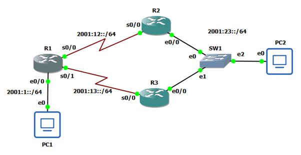
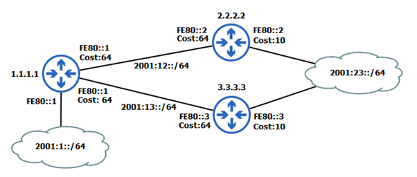
We will be using the same network topology, but the router interfaces have been configured with IPv6 addresses:
Let’s start the topology reconstruction process by examining the Router-LSA generated by R1:

The output shows some differences between the format of the Router-LSA in OSPFv3 and its counterpart in OSPFv2:
- The option field is longer (24 bits)
- The Link State ID is no longer equal to the RID of the advertising router
- All addressing information has been removed from the Router-LSA
- Link state information about interfaces connected to stub networks has been removed from the Router-LSA
In OSPFv3, a router may generate one or more Router-LSAs. Remember that the tuple LS type, Link State ID, and advertising router RID uniquely identifies an LSA in the Link State Database (LSDB). If more than one Router-LSA is generated, they can be distinguished by generating a different Link State ID for each of them.
In OSPFv2, both Router and Network-LSAs store some addressing information. Specifically, in the OSPFv2 Router-LSA we may find the following addressing information:
- For point-to-point links: Local interface IPv4 address
- For links connected to transit networks: DR interface IPv4 address and local interface IPv4 address
- For links connected to stub networks: Local interface IPv4 address and network mask
In OPSFv2, the network mask for transit networks is stored in the Network-LSA generated by the Designated Router (DR).
By contrast, OSPFv3 removes all addressing information originally stored in Router and Network-LSAs and moves it to other types of LSAs, as discussed later in this post. OSPFv3 router and network LSAs only contain the topological information necessary to build the Shortest Path First (SPF) tree. It means that Router and Network-LSAs are only flooded when a topological change occurs and prefix changes will not trigger any SPF recalculation, which is an improvement over OSPFv2.
The Router-LSA generated by R1 describes two point-to-point links:
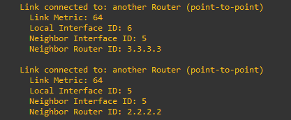
The fields used to describe the attached interfaces are:
- Metric
- Local Interface ID
- Neighbour Interface ID
- Neighbour Router ID
Metric represents the outbound cost assigned to the interface. Local Interface ID is a number that uniquely identifies the local router interface. Neighbour Interface ID corresponds to the interface ID of the neighbouring router and Neighbour Router ID identifies the node attached at the other end of the link.
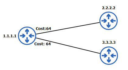
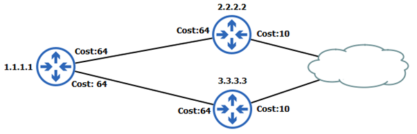
The two links described in the R1 Router-LSA can be translated into the following graph:
The neighbour RID can be used by the local router as a key to search in the LSDB for the next Router-LSA, to place another piece of the puzzle. Let’s examine both R2 and R3 Router-LSAs.
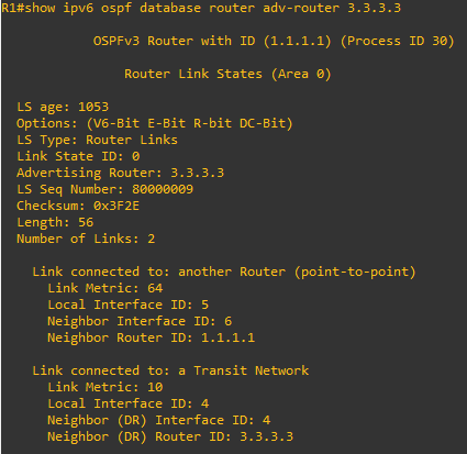
R3 router-LSA:
And R2 router-LSA:

These new Router-LSAs contain a link description that points back to R1. This link corresponds to the serial link that connects R1 to R2 and R3. These LSAs contain another interface type: ‘Link connected to a Transit Network’. The transit network corresponds to the ethernet segment that connects routers R2 and R3 through the switch SW1.
Like OSPFv2, OSPFv3 represents broadcast and nonbroadcast Multiaccess Networks (NBMA) by adding a pseudonode to the SPF topology. This pseudonode is described by a Network-LSA created by the DR, which is R3 in this topology. The Link State ID of a Network-LSA corresponds to the interface ID of the DR. This field, in combination with the RID of the DR, can be used as a key to search in the LSDB for the Network-LSA associated with the ethernet segment:
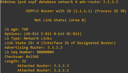
If we compare the previous output with the structure of a Network-LSA in OSPFv2, we may notice two main differences. First, the Link State ID field in OSPFv2 is equal to the IP address of the DR. In OSPFv3, this value is replaced by the interface ID of the DR, as mentioned before. Additionally, in OSPFv3 the network mask field is missing. Remember that the Router and Network-LSAs do not store any address information.
We can find information about prefixes and IPv6 addresses in the last two LSAs that need to be analysed to complete the starting network topology: Link and Intra-Area-Prefix-LSAs. But before moving on to the next LSAs, let’s add another piece to the puzzle using the information stored on the Network-LSA generated by R3:
Basically, the Network-LSA describes the list of routers connected to the same network segment (R2 and R3). The relationship between R2 and R3 can be described by the Network-LSA pseudonode, which is represented by the cloud in Figure 3. The cost to reach this pseudonode can be obtained from the Router-LSAs.
At this point, you may notice that Router and Network-LSAs provide all the topological information needed to build the SPF tree from any router to any other router. However, in addition to the topological information, routers need information about prefixes and neighbour link-local addresses to build their routing tables.
In OSPFv2, the next-hop IP address is determined from the Router-LSA received from the neighbouring routers. But Router-LSAs have an area flooding scope. Therefore, if an interface IP changes, a new Router-LSA is re-flooded throughout the entire area. But such change is only relevant to neighbouring routers connected to the same link where the interface is attached.
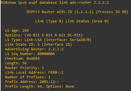
Another improvement of OSPFv3 over OSPFv2 is the addition of a link-local flooding scope. In OSPFv3, neighbour-specific information is placed in another LSA type: Link-LSAs. A router originates a separate Link-LSA for each attached link connected to one or more neighbours. A Link-LSA provides the following information:
- The router’s link-local address
- The list of IPv6 prefixes associated with the interface
- A collection of options bits (beyond the scope of this discussion)
Let’s examine the Link-LSA generated by R1 for its interface connected to the stub network where PC1 is attached:

From that output we can derive the following information:
- Link State ID: 4 (interface ID of R1 interface)
- Router Priority: 1
- Link Local Address: FE80::1
- Prefix associated with R1 interface: 2001:1::/64
The link-local scope of Link-LSAs can be confirmed by looking at the Link-LSAs generated by R2 from R1’s point of view:
The output shows that R1 receives only the Link-LSA from R2 associated with the point-to-point link between R1 and R2.
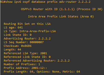
Finally, let’s examine the last LSA we will be discussing in this post: Intra-Area-Prefix LSA.
An Intra-Area-Prefix LSA provides a list of IPv6 prefixes that are associated with either a Router-LSA or a Network-LSA. A router may generate multiple Intra-Area-Prefix LSAs to keep the size of the LSA small. The different LSAs are distinguished by their Link State ID.
Let’s examine the Intra-Area-Prefix LSA generated by R1:

This LSA is linked to the R1’s Router-LSA by the fields: Referenced LSA Type, Referenced Link State ID, and Referenced Advertising Router. A total of three IPv6 address prefixes are described, which correspond to the two point-to-point links and the stub network.
If we examine the Intra-Area-Prefix LSAs generated by R3, we get the following output:
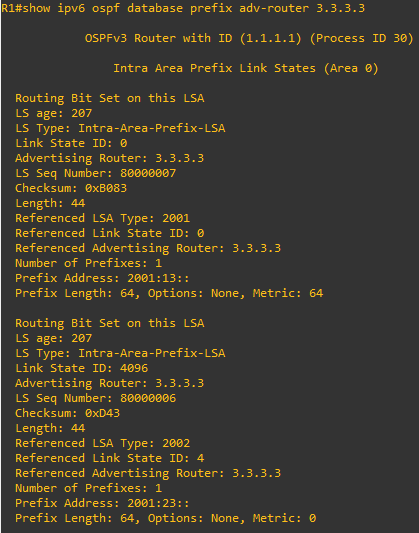
R3 generates two Intra-Area-Prefix LSAs: One for the point-to-point link to R1 and another for the transit network connecting R2 and R3. The Intra-Area-Prefix LSA associated with the transit network is linked to the Network-LSA generated by R3.
As a final note, let’s examine the output of the Intra-Area-Prefix LSA generated by R2:
This LSA only describes the IPv6 prefix associated with the point-to-point link connecting R1 to R2. R2’s Intra-Area-Prefix LSA omits the IPv6 prefix associated with the transit network because it is already described in the Intra-Area-Prefix-LSA generated by the DR.
Combining all the information from the different Link and Intra-Area-Prefix LSAs we can build the final topology:
Blas Trigueros is a Telecommunication Engineer who has worked in different IT areas since receiving his degree in 2005. He has experience as a developer and as a network administrator.
This post was adapted from the original at Networking Tales.
The views expressed by the authors of this blog are their own and do not necessarily reflect the views of APNIC. Please note a Code of Conduct applies to this blog.