

Statistical characterization of a Round Trip Time (RTT) series is useful for network management. For example, if several paths are available between a source and a destination, say in a routing overlay context, it may be useful to select the path dynamically based on some inference on the current Quality of Service (QoS) of each path.
In this post, we explain how the HDP-HMM can be used to model a RTT series and discuss possible applications of such modelling.
Statistical characterization of a RTT series
The Internet is an object of study itself and scientists want to characterize different metrics, in particular, QoS metrics (for example, delays, bandwidth or loss rates) with appropriate statistical models to improve their understanding of the Internet’s performance.
Because of the impact BGP routing configurations and load balancing have on the end-to-end QoS, an analysis of time-series Internet delays (such as RIPE Atlas RTT measurements) reveals a characteristic pattern of behaviour of these time series.
It is normally the case that, for a given origin-destination pair, RTTs take on a small set of different values with some random fluctuations around these few base values. The different values may correspond to different routing configurations resulting in different Internet paths from source to destination, whereas the random fluctuations may be due to congestion or measurement errors — RTT values switch from one base level to another after a few hours (Figure 1).
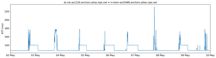
Figure 1 — RIPE Atlas RTT measurement between two RIPE Atlas anchors.
From a statistical point of view, this regularity can be explained by appropriate statistical models. We will show that HMMs, and more precisely HDP-HMMs, are appropriate stochastic models for the characterization of a RTT series, explain how the parameters of these models can be trained, and discuss what they can be useful for.
HMMs and model estimation
A Markov chain is a stochastic process in a way that the Markov property is satisfied. That means the current value of the process depends on the previous one only.
HMMs are ‘noisy versions’ of Markov chains: imagine a latent Markov chain, which is not observed directly, and observations that depend randomly on the latent Markov state. If we go back to our problem of a RTT series, modelling the different ‘base levels’ corresponds to the states x(t) of the Markov chain. RTT values correspond to observations y(t), or a trajectory of an HMM (Figure 2).
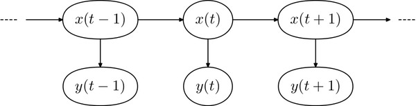
Figure 2 — Time evolution of an HMM, x(t) and y(t) are, respectively, the hidden states and noisy observation at time (t).
HMMs are parametric models. The stochastic model is specified by a few parameters only: the transition probabilities between states of the Markov chain, as well as the parameters of the probability distribution of observations given a particular state of the Markov chain (for example, means and variances under a Gaussian distribution assumption).
So, a first problem is to calibrate the model parameters from the measurements. The Expectation Maximization (EM) is a standard training algorithm for HMMs. But in practice, different problems are encountered when working with real datasets.
A first common issue with EM is that it converges to a local maximum of the likelihood of the observations, and this maximum may not be the global one if the EM has not been initialized very carefully.
A second problem is that the number of states of the Markov chain is often unknown (whereas it is supposed to be a known constant in EM).
For all these reasons we consider that a standard HMM model trained with EM is not a flexible enough approach to characterize RTT measurements. So far, several techniques have been proposed to cope with this problem. Recently, efficient generic methods have been developed to estimate HMM parameters, which offer more flexibility to capture the variability observed in different kinds of real datasets.
The Hierarchical Dirichlet Process HMM (HDP-HMM) builds on Bayesian inference. The number of states of the HMM, as well as the parameters of the probability distribution of observations in each state of the Markov chain, are considered as random variables.
In a Bayesian setting, a prior distribution is assumed for the parameters. Then, the distribution of the parameters conditioned on the observations, also known as the posterior likelihood, is the likelihood of the observations weighted by the prior distribution. Once this posterior distribution is obtained, it should be possible to obtain estimates of the parameters by looking at its mode or mean.
In practice, the exact computation of the posterior distribution is intractable. However, samples from this posterior distribution, that is to say, samples of the model parameters given a particular value of the set of observations, can be obtained using the MCMC (Markov Chain Monte Carlo) methods, in particular, Gibbs sampling. MCMC methods are classical stochastic simulation methods for Bayesian inference.
For complex data sets, the problem of estimating the number of states of an HMM is not straightforward. A possible approach is to use Dirichlet Processes (DP) as priors for the number of states, which makes it possible to specify that the number of states is finite but unknown.
Moreover, in order to introduce enough flexibility in the model and to be able to accurately fit various real datasets, HDP-HMMs are ‘hierarchical’. The model parameters (such as the transition probabilities of the Markov chain, and the means and variances of the Gaussian distributions of observations) depend on another layer of random variables and a ‘vague’ prior is set on this root layer of randomness. This hierarchy of random dependencies and vague priors introduces enough flexibility in the model to let it adapt to a much different time series, such as audio recordings or… RTT measurements!
Experiments on RIPE Atlas measurements
We at the IMT Atlantique, have explored this approach for the characterization of a RTT series using measurements from RIPE Atlas and an open-source implementation of HDP-HMM.
Built-in measurements between every RIPE Atlas anchor offers a comprehensive view of the QoS on the Internet: every 4 minutes, pings and traceroutes are executed for each pair of anchors. Using the RIPE Atlas API we have assembled a dataset of 81,000 series, representing IPv4 RTT measurements between every pair of anchors over one week. We considered the minimum value of the RTT at any given time slot, which resulted in 2,520 data points per series.
HMM parameters for each series have been learned using HDP-HMM. As a byproduct, the Gibbs algorithm, which has been used to fit parameters of the HDP-HMM model, also infers the underlying states associated with measured RTTs. Some results are displayed in Figure 3.
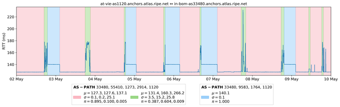
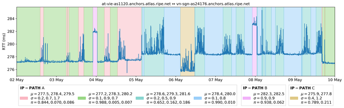
Figure 3 — States learned over a seven-day period for RTTs measured between two RIPE Atlas anchors.
Here, the same background colour corresponds to the same value of the latent Markov chain. So, observations that belong to the same ‘cluster’ are displayed on a background of the same colour. A visual inspection of many different clustering results has revealed that HDP-HMM is a very accurate model for the RIPE Atlas RTT time series. In particular, it is possible to split the RTT time series into a small, yet homogeneous, set of clusters.
One may wonder how many different states are necessary to characterize each origin-destination pair. So, we have processed a one-week long dataset of RTTs between all pairs of RIPE Atlas anchors. And for each pair of anchors, the number of states of the HDP-HMM model has been estimated. Figure 4 shows a histogram of the number of states obtained.
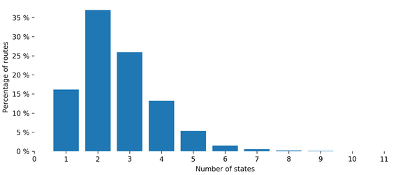
Figure 4 — Distribution of the number of states for models learned over one week.
For a vast majority of source-destination pairs, five or six states are more than enough to capture the variability in the distribution of RTTs on a one-week long time period. Fifty percent of the routes involve two or fewer states, and 99% six or less.
We then compared the number of states obtained on shorter timescales. Figure 5 displays the repartition of the number of states for periods of one day to one week.
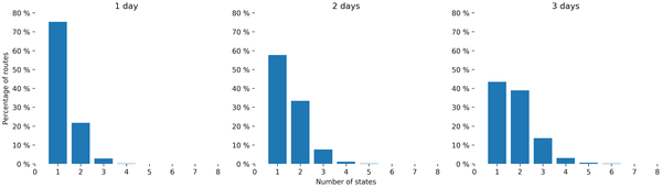
Figure 5 — Distribution of the number of states for different timeframes.
As one can expect, shorter periods lead to models with fewer states. Ninety-nine percent of the routes have four or fewer states for the two- and three-day long training periods, and three states or less for the one-day period.
Applications
You might wonder what this modelling is useful for, apart from intellectual satisfaction.
Well, first of all, it can be used to derive performance metrics: mean and variance of the RTT in each state, average sojourn time in each state, and probabilities of switching from one state to another, which can be more meaningful than global average performance metrics.
The proposed approach enables segmentation of the data with few persistent states, and rapidly detects changes of state. This avoids the many false alarms that would arise with some other detection approaches.
The performance of different paths can also be compared statistically. For example, computing the probability that the delay is larger on one path or another between one source and one destination is quite straightforward once an accurate stochastic model has been calibrated.
In our next post, we will investigate how such a model may be used for network management.
Contributors: Sandrine Vaton and Thierry Chonavel
Maxime Mouchet is a PhD student in Computer Science at IMT Atlantique (Brest, France) working on smart monitoring schemes for dynamic programmable networks.
The views expressed by the authors of this blog are their own and do not necessarily reflect the views of APNIC. Please note a Code of Conduct applies to this blog.