

Packet-switched networks benefit from buffers within the network’s switches.
In the simplest case, if two packets arrive at a switch at the same time and are destined to the same output port, then one packet will need to wait in a buffer while the other packet is sent on, assuming that the switch does not want to needlessly discard packets.
Not only do network buffers address such timing issues that are associated with multiplexing they are also useful in smoothing packet bursts and performing rate adaptation that is necessary when packet sources are self-clocked. If buffers are generally good and improve data throughput, then more (or larger) buffers are better, right?
This is not necessarily so, as buffers also add additional lag to a packet’s transit through the network. If you want to implement a low jitter service, then deep buffers are decidedly unfriendly! The result is the rather enigmatic observation that network buffers have to be as big as they need to be, but no bigger!
The Internet adds an additional dimension to this topic.
The majority of Internet traffic is still controlled by the rate adaptation mechanisms used by various forms of TCP congestion control protocols. The overall objective of these rate control mechanisms is to make efficient use of the network, such that there is no idle network resource when there is latent demand for more resource. And fair use of the network, such that if there are multiple flows within the network, then each flow will be given a proportionate share of the network’s resources, relative to the competing resource demands from other flows.
Buffers in a packet-switched communication network serve at least two purposes. They are used to impose some order on the highly erratic instantaneous packet rates that inherent when many diverse packet flows are multiplexed into a single transmission system. And to compensate for the propagation delay inherent in any congestion feedback control signal and the consequent coarseness of response to congestion events by end systems.
The study of buffer sizing is not one that occurs in isolation. The related areas of study encompass various forms of queueing disciplines used by these network elements, the congestion control protocols used by data senders and the mix of traffic that is brought to bear on the network. The area also encompasses considerations of hardware design, ASIC chip layouts, and the speed, cost and power requirements of switch hardware.
The topic of buffer sizing was the subject of a workshop at Stanford University in early December 2019. The workshop drew together academics, researchers, vendors and operators to look at this topic from their perspectives. It hosted 98 attendees from 12 economies with 26 from academia and 72 from industry. The following are my notes from this highly stimulating workshop.
Buffering 101
In an autonomously managed packet network, packet senders learn from reflections of data provided by packet receivers.
One aim of each packet sender is a position of stability, where every packet that is passed into the network is matched against a packet leaving the network. In the TCP context, this behaviour is termed ACK pacing.
Each ACK describes how many bytes were removed from the network by the receiver, which, in turn, can be used to guide how much additional data can be passed into the network.
The unknown factor in this model is that the sender is not aware of what is a fair and efficient amount of network resource to claim for the data transaction.
The TCP approach is to use a process of dynamic discovery where the sender probes the network with gently increasing sending rates until it receives an indication that the sending rate is too high. It then backs off its sending rate to a point that it believes is lower than this sustainable maximum rate and resumes the probe activity.
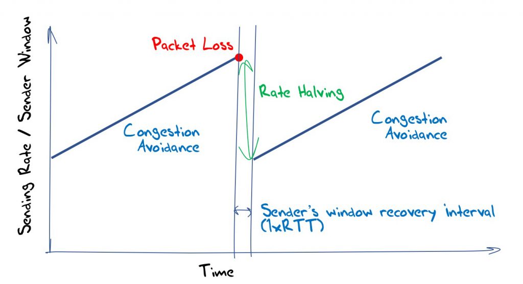
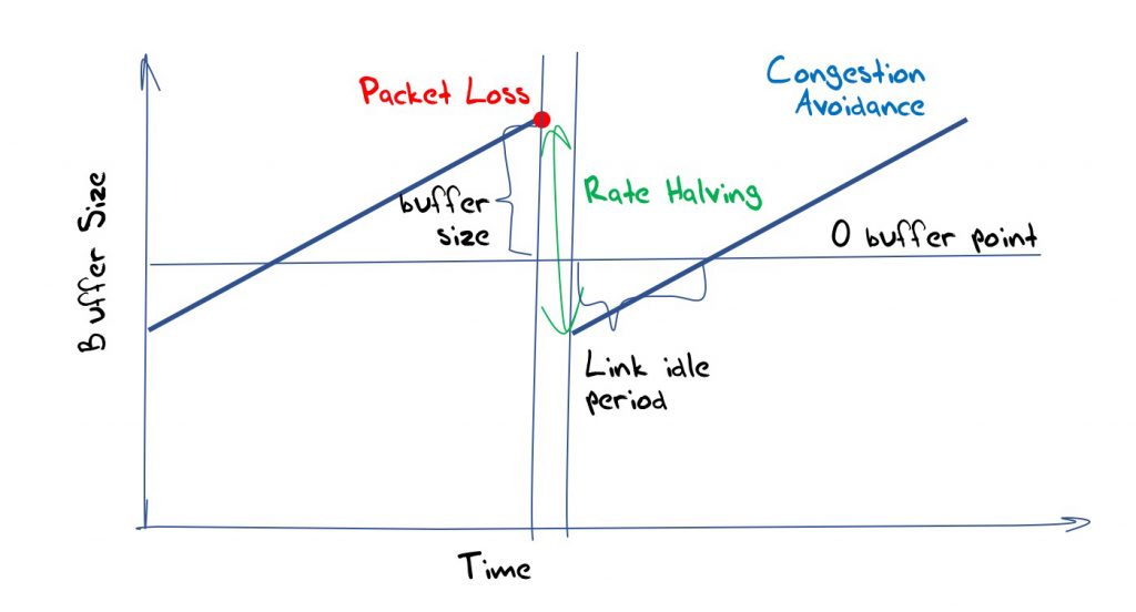
This classic model of TCP flow management is termed Additive Increase, Multiplicative Decrease (AIMD), where the sending rate is increased by a constant amount over each time interval (usually the time to send a packet to the receiver and send an acknowledgement packet, or a Round Trip Time (RTT)) and in response to packet loss event by decreasing the sending rate by a proportion. The classic model of TCP uses an additive factor of one packet per RTT and a rate halving (divide by two) in response to a packet loss. This results in a ‘sawtooth’ TCP behaviour (Figure 1).
If the packet loss function is assumed to be a random loss function with a probability p, then the flow rate is proportional to the inverse square root of the packet loss probability:
BW = ( MSS / RTT) ∙ (C / √p) where C = √(3/2)
This implies that the achievable capacity of an AIMD TCP flow is inversely proportional to the square root of the packet loss probability.
But packet loss is not a random event. If we assume that packet loss is the result of buffer overflow, then we need to also consider buffers and buffer depth in more detail.
An informal standard for the Internet is that the buffer size should be equal to the delay bandwidth product of the link (the derivation of this result is explained in the next section).
Size = BW ∙ RTT
As network link speeds increase, the associated buffers similarly need to increase in size, based on this engineering rule-of-thumb. The rapid progression of transmission systems from megabits per second to gigabits per second, and the prospect of moving to terabit systems in the near future, pose particular scaling issues for silicon-based switching and buffer systems.
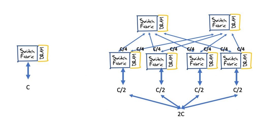
As networks increase in scale, then the switching scaling factors tend to show multiplicative properties. For example, if we have a single switch of capacity C and we would like to double the effective switching capacity but cannot increase the capacity of the switching chip, then how many switching chips are required to produce a composite switch of capacity 2C? The answer is not 2 but 6, as shown in Figure 2.
A packet will also need to traverse up to three switch fabrics so the aggregate buffer size of the path through the switch fabric may triple in size.
Self-clocking packet sources imply that congestion events within the network are inevitable, and any control mechanism that is imposed on these sources requires some form of feedback that will allow the source to craft an efficient response to congestion events.
However, this feedback is constrained by propagation delays and this lag creates some coarseness in the response mechanisms. If the response is too extreme the sources will overreact to congestion and the network will head into instability with oscillations between periods of intense use and high packet loss and periods of idle operation. If the response is too small the congestion events will extend over time, leading to protracted periods of operation with full buffers, high lag, and high packet loss.
Robust control algorithms need to be stable for general topologies with multiple constrained resources, and ways of achieving this are still the subject of investigation and experimentation. If feedback based on rate mismatch is available, then feedback based on queue size is not all that useful for stabilising long-lived flows. Feedback based on queue size is however important for clearing transient overloads.
Over more than three decades of experience with congestion management systems, we’ve seen many theories, papers and experiments. Clearly, there is no general agreement on a preferred path to take with congestion control systems. However, a consistent factor here is the network buffer size and the sizing of these buffers in relation to network capacity.
One view, possibly an extreme view, says that buffers are at the root of all performance issues.
The task of dimensioning buffers in a switching system has implications right down to the design of the ASIC that implements the switch fabric. The onboard memory can be fast but it’s limited in capacity to some 100MB or less. Larger memory buffers need to be provisioned off-chip, requiring I/O logic to interface to the memory bank and the speed of the off-board system is typically slower than onboard memory. Hybrid systems have to make a compromise between devoting chip capacity to switching, memory and external memory interfaces. And layered on top of these design trade-offs is the continuing need to switch at higher speed across larger numbers of ports.
One objective of this workshop was to continue the conversation about buffers, their relationship to congestion control and improve our understanding about the interdependence between buffer size, queuing control, self-clocking algorithms, network dimensioning and traffic profiles.
How big should a buffer be in the Internet?
The single AIMD flow model predicts poor outcomes for flows operating across buffers that are too deep or too shallow.
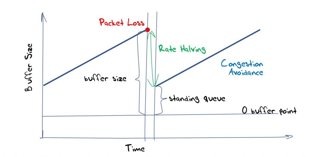
Too deep and the flow’s loss response of halving the congestion window does not clear the buffer and a standing queue forms that contributes to an increased latency imposed in the flow (Figure 3).
Too shallow and the rate halving drops the sending rate below the bottleneck capacity, and the link will be under-utilized until the additive increase brings the rate up to the link capacity (Figure 4).
The delay bandwidth product rule-of-thumb generates some extremely large queue capacity requirements in medium delay high capacity systems. A 10Gbs system using a 100ms RTT link requires a 125Mbyte memory pool per port that can read and write at 10Gbps. A 1T system would require a 12.5Gbyte memory pool per port, that can read and write at 1Tbps. A 16 port switch would require 200Gbytes of high-speed buffer memory using this same design guideline.
Such numbers are challenging for switch designers and it is reasonable to review the original work to understand the derivation of this provisioning rule. This model of provisioning the queue to the bandwidth-delay product is derived from an AIMD control algorithm of a single flow using an additive value of one segment per RTT and halving of the congestion window on packet loss, coupled with the objective of using the buffer to keep the link busy during the period of window deflation.
However, there is something a little deeper in the oscillation of the AIMD flow control process that impacts on the selection of the buffer size. In the purely hypothetical situation of a single flow operating across a single switch with a lossless transmission medium, the only source of packet loss is buffer exhaustion. If the switch has no buffer at all then the AIMD algorithm will operate in a steady-state between half capacity and full capacity, leaving approximately a quarter of the capacity unused by the flow.
The objective is to use a buffer as a reservoir to fill the transmission link while the sender has paused waiting for the receiver window to fall below the new value of the congestion window. If the buffer size is set to the link bandwidth times the link round trip time, then the buffer will be drained at the point when the sender will resume sending.
While this is a result from a theoretical analysis of a single flow through a single link, experiments by Villamizar and Song in 1994 pointed to the more general use of this dimensioning guideline in the case of multiple flows across multiple links. The rationale for this experimental observation was a supposition that synchronization occurs across the dominant TCP flows, and the aggregate behaviour of the elemental flows was similar to a single large flow. This was the foundation of today’s common assumption that buffers in the network should be provisioned at a size equal to the round-trip delay multiplied by the capacity to ensure efficient loading of the link.
This supposition has been subsequently questioned. The scenario of a link loaded with a diversity of flows in RTT, duration and burst profiles implies that synchronization across such flows is highly unlikely. This has obvious implications for buffer size calculation.
A study by a Stanford TCP research group in 2004 used the central limit theorem to point to a radically smaller model of buffer size. Link efficiency can be maintained for N desynchronized flows with a buffer that is dimensioned to the size of:
Size = (BW ∙ RTT) / √N
This is a radical result for high-speed extended latency links in a busy network. The consequences on router design are enormous:
“For example, a 1 Tb/s ISP router carrying one TCP flow with an RTTmin of 100ms would require 12.5 GB of buffer and off-chip buffering. If it carries 100,000 flows, then the buffer can be safely reduced to less than 40MB, reducing the buffering and worst-case latency by 99.7%. With small buffers, the buffer would comfortably fit on a single chip switch ASIC.”
Nick McKeown et. al. Sizing Router Buffers (Redux)
This background provides the backdrop of the Buffer Sizing Workshop.
Queue management
The default operation of a queue is to accept new packets while there is still space in the queue and discard all subsequently arriving packets until the output process has cleared space in the queue.
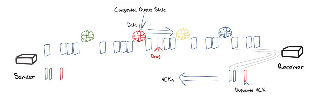
If an incoming packet burst arrives at a switch and there is insufficient queue capacity to hold the burst, then the tail of the burst will be discarded. This tail-drop behaviour can compromise the performance of the flow, as the clocking information for the tail end of the burst has been lost.
One mitigation of this behaviour is Active Queue Management (AQM), where queue formation triggers early drop. The ideal outcome is that packet drop in a large burst will occur inside the burst and the trailing packets following the drop point will carry a coherent clocking signal that will allow the flow to repair the loss quickly without losing the implicit clocking signal. Loss-based congestion control algorithms will react to this packet drop by dropping their congestion control window size, reducing their sending rate.
Delay-based paced control algorithms react differently to queue drop and the question is are there AQM functions which can support a mix of congestion control algorithms?
Indeed, is the question of what form of AQM to use a more important question than the size of the underlying buffer?
Explicit network feedback
For many years there has been considerable debate between an end-system approach that uses only the received ACK stream to infer the network congestion state in the data forwarding direction from a packet loss signal (Figure 5).
An approach that uses some form of explicit signalling from the network that can directly inform the source of the network state. Very early efforts in such direct signalling through ICMP Source Quench messages were quickly discounted due to the various issues related to its potential for DOS attack and inability to authenticate the message.
The Explicit Congestion Notification proposal tried to address the most obvious failing of the earlier approach by placing the congestion signal inside the end-to-end IP packet exchange. Switching elements that were experiencing the onset of local congestion load in their buffers were expected to set congestion experienced a bit in the IP packet header of packets that were contributing to this load condition. Receivers were expected to translate this bit into the ACK packet header so that the sender received an explicit congestion signal rather than having to infer congestion from an ACK signal that reflects packet loss (Figure 6).
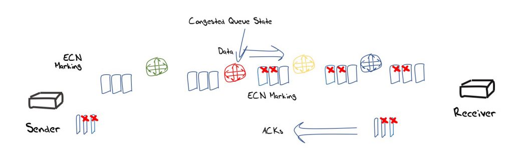
The advantage of ECN is that the sender is not placed in the position of being informed of a congestion condition well after the condition has occurred. Explicit notification allows the sender to be informed of a condition as it is forming so that it can take action while there is still a coherent ack pacing signal coming back from the receiver (that is before packet loss occurs).
However, ECN is only a single bit marking. Is this enough? Would a richer marking framework facilitate more precise sender response?
What if we look at a marking regime that marks based on the distance from the current rate to a desired fair efficient rate? Or use a larger vector to record the congestion state in multiple queues on the path?
The conclusion from one presentation is that the single-bit marking, while coarse and non-specific is probably sufficient to moderate self-clocking TCP flows such that they do not place pressure on network buffers, leaving the buffers to deal with short term bursts from unconstrained sources.
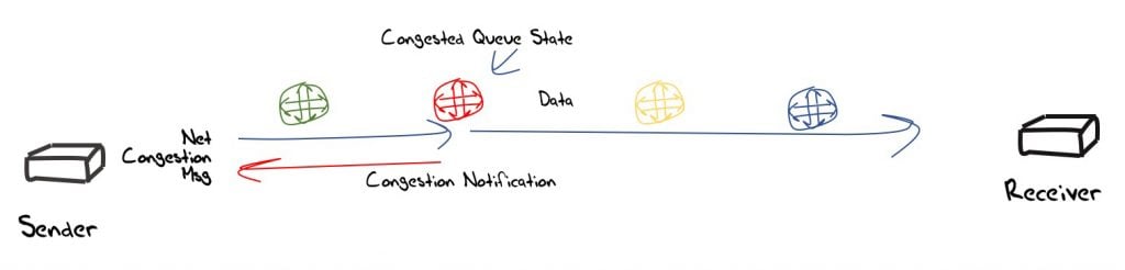
Another presentation explored a network-level direct feedback message, analogous to the ICMP Packet Too Big messages in path MTU discovery. To short-circuit the delays associated with completing the entire round trip, this approach envisages the switch experiencing the onset of congestion to explicitly message the source of this congestion condition (Figure 7).
Another presentation looked at the attachment of a detailed telemetry log to each packet in a data centre application.
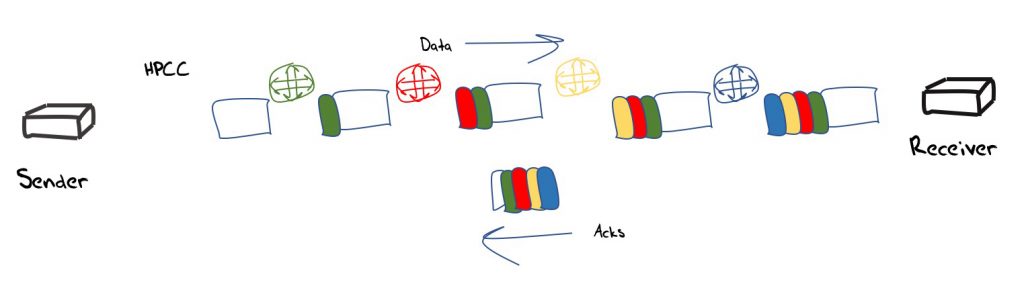
In the High Precision Congestion Control (HPCC) framework each switch attaches the time, queue length, byte count and link bandwidth to the data packet. The receiver takes this data and attaches it to the corresponding ACK, so that the sender can form a detailed model of the recent state of path capability.
HPCC allows the sender to calculate a fair sending rate and then rapidly converge to this rate, while at the same time bounding the formatting of queues and bounding queuing delays. The domain of application of this approach appears to be the data centre and the objective is to achieve high speed with bounded delay for remote direct memory access (RDMA)-style applications (Figure 8).
There is a degree of debate between congestion-based TCP control and delay-based mechanisms. On the one hand, we hear that delay-based mechanisms can operate the flows at the onset of queue formation in the network. On the other hand, we hear that attempting to set the flow to a fixed delay and operating with fairness to other flows is intrinsically impossible and that we need to operate flows with congestion moderation.
Near and far buffers
What is the cost/power trade-off of buffers on-chip and off-chip? And if we are considering off-chip what do we mean, as there are different implementation approaches to off-chip memory?
As a general observation, the performance of off-chip memory is not remotely close to what is required by a high capacity high-speed switch. This is not improving over time as memory speed is not scaling at the same rate as transmission and even switch speeds, so the gap in performance between transmission and switching and memory speed is only getting larger over time.
One switch chip fabricator, Broadcom, implements both deep and shallow buffers. On their switch fabric chip, they use small fast buffers and wrap the switch fabric with everything they can to reduce the dependency on deep buffers.
The picture from Intel is that a lot of recent data suggests that shallow buffers may be good enough. But due to limitations in instrumenting technologies, there is insufficient confidence in these results to allow switch chip designs to completely do away with external memory interfaces and a local cache and use on-chip memory exclusively.
Current switch designs use between 10% to 50% of the chip area on memory management. This observation applies to high capacity high-speed switches because at a lower capacity and lower speeds there is no such constraint, and large pools of off-chip memory (relative to transmission speeds) can be used; although some constraint in the amount of memory will likely produce a better outcome in these contexts as well.
The question of future requirements that is always present in chip design, given the long times between phrasing requirements and deployment into networks, is where is this heading?
Memory buffers are not growing as fast as chip bandwidth. Clock speeds are not increasing. And scaling chip bandwidth has currently achieved parallelism rather than increasing the chip’s clock speed. While doubling switch capacity may be feasible, contemplating an increase in capacity by factors of 20, 50 or even 100 seem like particularly tough challenges.
Today, packet rates are typically achieved with multiple parallel pipelines and orchestrating such highly parallel mechanisms creates its own complexity in design. No one is yet prepared to call an end to the prodigious outcomes of Moore’s Law in the semiconductor realm, but it looks like clock speeds are not keeping up. Pin density and even increasing gate density is becoming challenging.
Is doubling the number of ports on a switch chip good enough? If a chip has twice the switch bandwidth does it need twice the on-chip memory capacity? Or less? The answer lies in external factors such as congestion control algorithms, queue management disciplines and delay management.
Hop-by-hop flow control
This is a revival of a very early attribute of packet-switched networks, where an end-to-end path is composed of a sequence of flow-controlled hops.
Each switching element sends at its line rate and sends into the buffer of the next switch. When a queue forms at the receiver the hop flow control can pause the flow coming from the adjacent switch and resume it when the queue is cleared.
Yes, this sounds very reminiscent of X.25 and the DDCMP component of DECnet, and it’s the opposite of the intent of the end-to-end approach. However, the approach can produce direct back-pressure on a bursting source with no packet drop and yield highly efficient use without extensive buffer-induced delays. Essentially the self-clocking nature of the flow is replaced with a network clocking function (Figure 9).
Admittedly, this is not a universally applicable approach, and it appears to offer a potential match to the intra-datacentre environment where traffic patterns are highly bursty, propagation times are low, paths are short, and volumes and speeds are intense.
Flow-aware buffer management
It appears that the move towards shorter buffers relative to the link speed is inevitable. But how to manage the feedback systems to allow self-clocking data sources to adjust to the shortened buffer space is still an outstanding issue.
One approach starts with a basic traffic characterisation of a relatively small proportion of ‘elephant flows’ (high volume, long duration) mixed with a far higher count of ‘mice’ flows (low volume, short duration). While elephant flows are highly susceptible to congestion signalling, mice flows are not.
If the network was in a position to be able to classify all currently active flows into either elephants or mice, then the network could be able to use different queuing regimes for each traffic class. This sorting adds to the cost and complexity of packet switches, and if scaling pressures are a factor in switch design then it’s not clear that the additional cost of switch complexity would be offset by a far superior efficiency outcome in the switching function.
Assuming that such a flow classification could be achieved dynamically, then differential responses can be contemplated.
For short flows, there is little benefit to be gained by any form of explicit congestion control other than placing all such flows into their own queuing regime.
For long-lived large flows, an explicit network congestion signal could be contemplated. This could take the form of an explicit packet back to the source generated by the network. The advantage of this approach is that the feedback of excessive sending rate is faster than a full RTT interval, allowing a timely response by the sender. However, this does seem like a reprise of the ill-fated ICMP Source Quench message, and all that was problematical with ICMP Source Quench is probably still an issue in this form of network congestion notification
This concept of the use of various queue regimes for different flow types can be exploited differently, using a short buffer for long flows in the expectation that the implicit congestion signal of packet drop would allow the long duration flow to stabilize into the available network resource, while short unregulated bursts could have access to a deeper buffer allowing the buffer to be used effectively as a rate adaptation tool to mitigate the burst.
This is taken even further in one project, that used the observation that if a buffer is too deep then the flow rate reduction following packet drop will leave a standing queue in the buffer, and if the buffer is too shallow then the rate reduction will leave a period of an empty queue and an idle transmission system. This observation means that a flow aware buffer manager could adjust its buffer size following observation of the post-reduction behaviour, reducing the buffer if standing queues form and increasing it if the queue is idle.
It’s an interesting approach to fair queuing flow management, treating the per-flow buffer as an elastic resource that can resize itself to adapt to the flow’s congestion management discipline.
ISP network buffer profile
P4 is a language used to program the data plane of network devices. The language can express how a switch should process packets (P4 itself comes from the original paper that introduced the language, Programming Protocol-independent Packet Processors.)
Barefoot’s Tofino is an example of a new class of programmable Ethernet packet switches that are controlled through P4 constructs, and these units can currently handle some 12.8Tbps of data plane capacity. What this allows is a measurement regime that can expose packet characteristics at a nanosecond level of granularity.
By tapping the packet flow of a high-speed trunk transmission system into and out of a switching element in the network and attaching the taps to a P4 switch unit it is possible to match the times of ingress and egress of individual packets and generate a per-packet record of queuing delay within the switching element at a nanosecond level of granularity. This provides a new level of insight into burst behaviour in high-speed carriage systems used by ISPs.
The major observation from an exercise conducted on a large ISP network was that network buffers are lightly used except for ‘microbursts’. These are bursts of some 100 microseconds or so, where the queue adds a delay element of more than 10ms on a 10G port.
Further analysis reveals an estimate of packet drop rates if the network’s buffers were reduced in size, and for this particular case, the analysis revealed that an 18msec buffer would be able to sustain a packet drop rate of less than 0.005%.
If buffer congestion behaviours in such ISP networks are in fact microbursts then network measurement tools that operate at the per-minute or even at the per-second level of granularity are simply too crude.
P4-based measurements that can resolve behaviours at the nanosecond level offer new insights into buffer behaviours in networks that carry a large volume of diverse flows. Even though the per-flow control cycle of the data plane flows is of the scale of some milliseconds and longer, the microburst behaviour is that of a load model that exhibits sub-millisecond bustiness. The timescale of end-to-end congestion control operates at a far coarser level than the observed behaviour of congestion within a switch running a conventional traffic load.
This leads to the observation that large-scale systems are creating extremely rapid queue size fluctuations and it is unrealistic to expect that end-to-end control algorithms can control the queue size. It might be that at best these control algorithms can contribute to influencing the distribution of queue sizes.
Sender pacing
The Internet can be seen as a process of statistical multiplexing of a collection of self-clocked packet flows where the flows exhibit a high degree of variance and a low level of stability.
The reaction to this unconstrained input condition so far is to use large buffers that can absorb the variations in traffic. How large is ‘large enough’ becomes a critical question in such an environment.
The work on buffer sizing as being in proportion to the bandwidth-delay product of the transmission elements is an outcome of a process that measures the properties of the control algorithm for traffic flows and then derive estimates of buffer sizes that should be capable of carrying such a volume of traffic that will efficiently and fairly load the transmission system.
The exercise assumes that the buffer dimension is a free parameter in network design and control algorithms are fixed. Buffer speed inside the network has to double at a cycle of some two years, and the buffer size has to double in a similar time frame. The product of size and speed is a quadrupling every two years.
The current tactical response to this escalation of buffer requirements due to transmission capacity increases has been to reduce the size of the buffers relative to the transmission capacity. However, this is not a long-term sustainable response as such under-provisioned network buffers will impair overall network efficiency in these self-clocking flow regimes.
The prospects for self-clocked traffic flows are not looking all that bright given that the growing demands for network buffer-based mitigation of unconstrained sender behaviours appear to be more than what can be satisfied within constraints of the constant unit cost of network infrastructure. Without overall economies of scale where larger service delivery systems achieve lower unit costs of service delivery, the management of traffic and content assume a different trajectory that tends to drive towards greater distribution and dispersal rather than continued aggregation and amalgamation. For the large hyper-scale content enterprises in today’s Internet, this is not exactly the optimal outcome.
It is a potentially fruitful thought process to look at this from an inverted perspective and look at the desirable control algorithm behaviour that makes efficient use of the network’s transmission resources when the available buffering is highly restricted. This thought process leads to the consideration of ‘pacing’ where the server uses high precision timers to smooth data flows as they leave the server, attempting to create a stable traffic flow that matches bottleneck capacity on the path. The more accurate this estimation of bottleneck bandwidth, the lower the demand for buffer capacity due to burst adaptation.
Residual buffer demand is presumably based on the demands of statistical multiplexing of disjoint flows. Given that the senders are under the control of the service delivery platforms and there are orders of magnitude fewer high-volume senders than receivers, this form of change is actually far less than the change required by, say, the IPv6 transition.
It is this thinking that lies behind the BBR protocol work. The sender’s flow control algorithm generates an estimate of the bottleneck bandwidth and the minimum RTT interval and then paces packet delivery to exactly feed traffic into the bottleneck at the bottleneck capacity, which should not involve the formation of a queue at the bottleneck.
The BBR control algorithm periodically probes up to revise its previous bandwidth estimate, and probes down to revise its previous minimum RTT, and takes into account other congestion formation signals, such as ECN. This probing up and down, or ‘dithering’, is not precisely specified in the core BBR algorithm and these parameters are being revised in the light of deployment experience to determine dithering settings that are both efficient and fair. The expectation is that BBR will not drive the formation of standing queues in the network and will pace the flow at the maximal rate that can be fairly sustained by the network path.
However, BBR is not the only way to perform flow pacing and there are still a large number of outstanding questions. How does pacing at the sender impact on the queue management at the edge close to the client? What are the cross impacts of burst traffic with pacing? How should a pacing control algorithm react to packet loss? Or out of order packet delivery? Can strict flow pinning still be required for ECMP or does pacing relax such requirements for strict path pinning? Are pacing or self-clocking the only options, or are the other approaches?
One perspective is that we are sitting between two constraint sets. Escalating volume and speed in the core parts of the network imply that bandwidth-delay product model buffer sizing is an unsustainable approach. The scaling back of buffer sizes in the network means that self-clocked protocols will potentially become more unstable and compromise achievable network efficiency and fairness. From this perspective, sender pacing looks to be a promising direction to pursue.
Is there a buffer sizing problem?
In the Internet, we are currently seeing a diversity of responses to network provisioning.
Some network operators use equipment with generous buffers. These buffers are overly generous according to the buffer bloat argument. Other network operators field equipment with scant buffers that run the risk of starving data sources while leaving idle network capacity.
There is a mix of congestion control algorithms (CUBIC, NewRENO, BBR, LEDBAT) and a mix of queue management regimes (CODEL, RED, WRED). There is a diversity of deployment environments, including mobile networks, Wi-Fi, wired access systems, LANs, and data centres. And there is a mix of parameters of the desired objective here, whether it’s some form of fairness, loss, jitter, start-up speed, steady-state throughput, stability, efficiency, or any combination of these factors. It is little wonder that its challenging to formulate a clear picture of common objectives and to determine what actions are needed to achieve whatever it might be that we might want!
There is the assumption that large network buffers absorb imprecision in clocking (timing ‘slop’) and allow simpler coarser rate control algorithms to operate effectively without needing high precision tuning.
Small network buffers provide little leeway and tolerance for such approximate approaches.
This mistrust of the level of precision of control exercised by end systems is a pervasive view within the networking community, and it could even be characterized as an entrenched view. So entrenched is this view that there is probably no experimental result that could convince the community as a whole that network buffers can be far smaller than they are today, all other things being equal.
This is despite the overwhelming evidence that overly large buffers compromise network performance, a position that has been described as ‘buffer bloat’. There are other reasons why large buffers are a problem for networks and users.
As we scale up the size and speed of the network large very high-speed buffers are also increasing in cost. If we are going to admit compromises and trade-offs in network design, is reducing the relative size of the buffer an acceptable trade-off?
And if we want to reduce buffer size and maintain efficient and fair performance how can we achieve it?
One view is that sender pacing can remove much of the pressure on buffers, and self-clocking flows can stabilise without emitting transient bursts that need to be absorbed by buffers. Another view, and one that does not necessarily contradict the first, is that the self-clocking algorithm can operate with higher precision if there was some form of feedback from the network on the state of the network path. This can be as simple as a single bit (ECN) or a complete trace of path element queue state (HPCC).
This remains a rich area of unanswered questions: What does it imply when the time scale of buffer congestion events is orders of magnitude smaller than the timescale of self-clocking flows? Are flows overly reliant on loss signals and too insensitive to delay variation? Can paced delay-based algorithms like BBR coexist with loss based oscillating algorithms such as CUBIC and new Reno? Would the general adoption of sender pacing change the picture of buffer sizing in the Internet?
How big should buffers be in the network? Or perhaps the opposite is the more practical question. How small can we provision buffers in an increasingly faster and larger network and still achieve efficient and fair outcomes in a variety of deployment environments?
All good questions for further research, experimentation and measurement.
The views expressed by the authors of this blog are their own and do not necessarily reflect the views of APNIC. Please note a Code of Conduct applies to this blog.
I wish I’d presented at this conference; now that I understand the typical arguments better.
one: is for large numbers of well mixed flows I generally buy the stanford sqrt(n) argument or less for buffer sizing. Secondly with the rise of fq_X (where X is codel, pie, or cake), we not only get perfect sharing and mixing but an independently calculated bdp per flow sufficient to keep flows of nearly any given rtt holding an equal share of that bottleneck.
Another thing that the codel algorithm does that is ill-understood is drop head queuing, which signals congestion faster and usually supplies the next packet in the flow immediately so the hole can be noticed and filled in faster.
Pacing improves mixing and creates an implicit more fq’d and fate sharing environment.
drop tail FIFOs must die, and perhaps if more folk were experimenting with rfc8290 in more scenarios, and ecn, perhaps we could put some of this argument over buffer size down in favor of smarter buffers.
Nice overview article for the buffer sizing problem. I wanted to briefly note two (probably common) misconceptions:
1) The legend “Rate Halving” is unfortunately incorrect in figures 4 and 5: “Window Halving” would be correct. Note that the effective RTT is inflated by the queuing delay caused by the standing queue in the bottleneck buffer. If one assumes a BDP-sized buffer, the average sending rate when the loss occurs is R=CWND_loss/RTT_eff=2BDP/RTT_eff=2BDP/(2RTT_base), .i.e.,
exactly the same when the sender continues to send new segments and the buffer has fully drained R=BDP/RTT_base, where RTT_base is the RTT without any queuing delay. This means that the average sending rate is not halved, but stays the same after a packet loss. That’s why a Buffer/Standing queue of 1 BDP is optimal for loss-based CC and a backoff factor of 0.5.
2) The standing queue explanation and legend in Figure 4 are not quite correct. Using the definition from the Codel Paper (https://queue.acm.org/detail.cfm?id=2209336) “The standing queue has nothing to do with the sender’s rate but rather with how much the sender’s window exceeds the pipe size. This standing queue, resulting from a mismatch between the window and pipe size, is the essence of bufferbloat.” (see also caption of Figure 4 in the Codel Paper). The good queue would dissipate within an RTT_base, the bad queue (standing queue) would persist for several RTTs, i.e., the standing queue is actually built up by TCP when growing linearly into the buffer in figures 4 and 5, so it is always the full buffer content (and not only the part that is not drained after the backoff) unless it dissipates within an RTT_base.
I have been trying to include limit – buffer size through netem (a linux network emulator). For the experiment I set the network profile on my bridge node as
” sudo tc qdisc add dev netw0 root netem rate 100mbit delay 10ms limit 41″
limit=(100*1000/8)/(1500)*10)/2)
I calculated the limit with the formula I found on stackoverflow but so far it doesn’t seems right when it comes to anomalies of various kinds. is there any other optimal way to calculate limit where we can set bandwidth rate, I do have 1gbps network bandwidth but I want to limit it based on bandwidth rate i provide